

Chapter 9: Sensitivity Analysis

Key Takeaways
- The Improve Conditions and Performance scenario is highly sensitive to the real discount rate assumed in the analysis. Substituting in a 3-percent discount rate for the 7-percent discount rate assumed in the baseline would increase its average annual investment requirements by 28.2 percent.
- Both HERS and NBIAS are more sensitive to changes in the assumed value of time than to the assumed value of a statistical life.
- Directly applying the future traffic projections reported by States via HPMS and NBI would increase the average annual investment levels for both the Maintain Conditions and Performance and Improve Conditions and Performance scenarios by approximately 10 percent, relative to the baseline VMT growth assumption derived from a national VMT forecasting model.
Highway Sensitivity Analysis
Sound practice in investment modeling includes analyzing the sensitivity of key results to changes in the underlying assumptions. For the Maintain Conditions and Performance scenario and the Improve Conditions and Performance scenario presented in Chapter 7, this section analyzes how changes in some of the underlying assumptions would affect the estimate of the average annual levels of highway investment. Some of the key economic assumptions include:
- value of traveler time savings in the 2014 base year,
- value of statistical life,
- discount rate used to convert future costs and benefits into present-value equivalents, and
- projected growth in aggregate traffic volumes.
An important outcome of the HERS results is that, under both baseline and sensitivity test assumptions, the Maintain Conditions and Performance scenario is equivalent to one in which the metric to be maintained is simply average pavement roughness. As defined, the Maintain Conditions and Performance scenario sets HERS-related spending at the lowest level at which the 2034 projections for each of two measures—the average International Roughness Index (IRI) and average delay per vehicle miles traveled (VMT)—indicate conditions and performance that match or surpass those in the 2014 base year. In each of this report’s simulations of this scenario, however, the binding constraint was to maintain average IRI. (The level of HERS-related spending that just sufficed to meet this constraint resulted in a decrease in average delay per VMT below the level in 2014.) For this reason, and because travel time delay depends much more on highway capacity than on pavement condition, any change to HERS assumptions that causes the model to reduce the share of spending for system expansion projects also will decrease the HERS component of spending in the Maintain Conditions and Performance scenario (and vice versa).
Alternative Economic Analysis Assumptions
For application in benefit-cost analyses of programs and actions under their purview, the U.S. Department of Transportation (DOT) periodically issues guidance on valuing changes in travel time and traveler safety, and the Office of Management and Budget (OMB) provides guidance on the discount rate to be used. Recognizing the uncertainty regarding these values, the guidance documents include both specific recommended values and ranges of values to be tested. The analyses presented in Chapters 7 and 10 of this report are based on the primary recommendations in DOT and OMB guidance for these economic inputs, whereas the analyses presented in this chapter rely on recommended alternative values to be used for sensitivity testing.
Value of Travel Time Savings
The value of travel time savings is a key parameter in benefit-cost analysis of transportation investments. For HERS and NBIAS, the Federal Highway Administration (FHWA) estimates average values per vehicle hour traveled by vehicle type. Primarily, these values reflect the benefits from savings in the time travelers spend in vehicles, also taking into account that vehicles can have multiple occupants. Time used for travel represents a cost to society and the economy because that time could be used for other more enjoyable or productive purposes. For heavy trucks, FHWA makes additional allowances for the benefits from freight arriving at its destination faster and from the opportunities for more intensive vehicle utilization when trips can be accomplished in less time. Even for these types of vehicles, however, the value of travel time savings estimated by FHWA primarily reflects the benefits from the freeing of travelers’ time—the time of the truck driver and other vehicle occupants.
For valuation of traveler time, the analysis in this report follows DOT’s guidance on valuing travel time saved in 2014. In the analyses presented in Chapters 7 and 10, traveler time savings are valued per person hour at $12.30 for personal travel and between $27 and $32 for business travel. The value for personal travel is set in the guidance at 50 percent of hourly household income, calculated as median annual household income divided by 2,080, the annual work hours of someone working 40 hours every week. The values for business travel are set at the relevant estimate of average hourly labor compensation (wages plus supplements). The variation in these values by vehicle type indicates, for example, that truck drivers typically earn less than business travelers in light-duty vehicles. (For details on the derivation of these values, see Appendix A.)
These values per person hour of travel are estimates subject to considerable uncertainty. Even when personal and business travel purposes are distinguished, estimating an average value of travel time is complicated by substantial variation in the value of travel time among individuals and, even for a given individual, among trips. Contributing to such variation are differences in incomes, employment status and earnings, attitudes, conditions of travel (e.g., the level of traffic congestion), and other factors. Moreover, studies that estimate values of travel time often are difficult to compare because of differences in data and methodology.
In view of these uncertainties, DOT guidance calls for sensitivity tests that set values of travel time lower or higher than for the baseline. For personal travel time, these values are 35 percent and 60 percent of median hourly household income, rather than 50 percent as assumed in the baseline. For business travel time, these values are 80 percent and 120 percent of average hourly labor compensation, rather than the baseline assumption of 100 percent.
Exhibit 9-1 shows the effects of these variations on spending levels in the two scenarios reexamined in this chapter. For the NBIAS-derived component of spending, the effects are small (at most 2.1 percent), consistent with bridge capacity expansion being outside the model’s scope. Except where they would eliminate long detours caused by vehicle weight restrictions on a bridge, the bridge preservation actions evaluated by NBIAS would have minimal effect on travel times.
For the HERS-derived component of spending, the percentage reductions with lower values of traveler time are close to 6 percent in the Maintain Conditions scenario and 10 percent in the Improve Conditions scenario. In the Improve Conditions and Performance scenario, the goal is to exploit all opportunities for cost-beneficial investments, which become fewer when the travel time savings are valued less. In the Maintain Conditions and Performance scenario, valuing travel time savings less decreases the share of spending that HERS allocates to capacity expansion, making funds available for the system preservation improvements that reduce pavement roughness. For this reason, and because the binding constraint in this scenario is maintaining average pavement roughness, the required level of HERS-related spending decreases. Conversely, that spending increases when the higher values of time are assumed.
Exhibit 9-1: Impact of Alternative Value of Time Assumptions on Highway Investment Scenario Average Annual Investment Levels
| Maintain Conditions and Performance Scenario | Improve Conditions and Performance Scenario | |||
|---|---|---|---|---|
| Alternative Time Valuation Assumptions for Personal and Business Travel as Percentage of Hourly Earnings | Billions of 2014 Dollars | Percent Change From Baseline | Billions of 2014 Dollars | Percent Change From Baseline |
| Baseline1 (Personal–50%; Business–100%) | $102.4 | $135.7 | ||
| HERS-Derived Component | $59.5 | $73.2 | ||
| NBIAS-Derived Component | $12.9 | $22.7 | ||
| Other (Nonmodeled) Component | $30.0 | $39.8 | ||
| Lower (Personal–35%; Business–80%) | $97.2 | -5.0% | $124.8 | -8.0% |
| HERS-Derived Component | $56.0 | -5.9% | $66.0 | -9.9% |
| NBIAS-Derived Component | $12.7 | -1.2% | $22.2 | -2.1% |
| Other (Nonmodeled) Component | $28.5 | -5.0% | $36.6 | -8.0% |
| Higher (Personal–60%; Business–120%) | $106.7 | 4.2% | $143.8 | 5.9% |
| HERS-Derived Component | $62.4 | 4.9% | $78.6 | 7.3% |
| NBIAS-Derived Component | $13.1 | 1.3% | $23.0 | 1.3% |
| Other (Nonmodeled) Component | $31.3 | 4.2% | $42.1 | 5.9% |
1 The baseline levels shown correspond to the systemwide scenarios presented in Chapter 7. The investment levels shown are average annual values for the period from 2015 through 2034.
Sources: Highway Economic Requirements System and National Bridge Investment Analysis System.
Nonmodeled Highway Investments
The HERS-derived component of each scenario represents spending on pavement rehabilitation and capacity expansion on Federal-aid highways. The NBIAS-derived component represents rehabilitation spending on all bridges, including those off the Federal-aid highways. The nonmodeled component corresponds to system enhancement spending, plus pavement rehabilitation and capacity expansion on roads not classified as Federal-aid highways.
In the Sustain 2014 Spending scenario presented in Chapter 7, the values for these HERS and NBIAS components sum to $74.6 billion. In 2014, nonmodeled spending accounted for 29.3 percent of total investment and is assumed to form the same share in all scenarios presented in Chapter 7.
Likewise, for the sensitivity analysis for the Maintain Condition and Performance and the Improve Condition and Performance scenarios presented in this section, the nonmodeled component is set at 29.3 percent of the total investment level. As the combined levels of the HERS-derived and NBIAS-derived scenario components increase or decrease, the nonmodeled component changes proportionally. Consequently, the percentage change in the nonmodeled component of each alternative scenario relative to the baseline always matches the percentage change in the total investment level for that scenario.
Value of Traveler Safety
One of the most challenging questions in benefit-cost analysis is what monetary cost to place on injuries of various severities. Few people would consider any amount of money to be adequate compensation for a person’s being seriously injured, much less killed. On the other hand, people can attach a value to changes in their risk of suffering an injury, and indeed such valuations are implicit in their everyday choices. For example, a traveler may face a choice between two travel options that are equivalent except that one carries a lower risk of fatal injury but costs more. If the additional cost is $1, a traveler who selects the safer option is manifestly willing to pay at least $1 for the added safety—what economists call “revealed preference.” Moreover, if the difference in risk is, say, one in a million, then a million travelers who select the safer option are collectively willing to pay at least $1 million for a risk reduction that statistically can be expected to save one of their lives. In this sense, the “value of a statistical life” among this population is at least $1 million.
Based on the results of various studies of individual choices involving money versus safety tradeoffs, some government agencies estimate an average value of a statistical life for use in their regulatory and investment analyses. Although agencies generally base their estimates on a synthesis of evidence from various studies, the decision as to which value is most representative is never clear-cut, thus warranting sensitivity analysis. DOT issued guidance in 2014 recommending a value of $9.4 million for analyses with a base year of 2014, as is the case in this C&P Report. The guidance also required that regulatory and investment analyses include sensitivity tests using alternative values of $5.2 million as the lower bound and $13.0 million for the upper bound. For nonfatal injuries, the guidance sets values per statistical injury as percentages of the value of a statistical life; these vary by the level of severity, from 0.3 percent for a “minor” injury to 59.3 percent for a “critical” injury. (The injury levels are from the Maximum Abbreviated Injury Scale.)
Impact of Alternatives on HERS Results
HERS contains equations for each highway functional class to predict crash rates per VMT and parameters to determine the number of fatalities and nonfatal injuries per crash. The model assigns to crashes involving fatalities and other injuries an average cost consistent with DOT guidance, including the use of alternative values for sensitivity tests. As shown in Exhibit 9-2, the sensitivity tests reveal only minor impacts on the average annual requirement for HERS-related investment; relative to a baseline in which the value of a statistical life is set at $9.4 million, increasing or decreasing that value by about $3.9 million alters the estimated investment requirement by well under 2 percent in each case. One reason for this relative insensitivity is that crash costs are estimated in HERS to form a small share of total highway user costs. In addition, from Chapter 10’s discussion of “Impact of Future Investment on Highway User Costs,” it emerges that the crash costs are less sensitive than travel time and vehicle operating costs to changes in the level of total investment within the scope of HERS. (Data limitations preclude that scope from including highway improvements that primarily target safety issues.) For NBIAS-related investment, the sensitivity of the estimated annual spending requirement to the tested variations in the value of a statistical life is even less than for HERS-related investment.
Exhibit 9-2: Impact of Alternative Value of a Statistical Life Assumptions on Highway Investment Scenario Average Annual Investment Levels
| Alternative Value of Statistical Life Assumptions (2014 Dollars) | Maintain Conditions and Performance Scenario | Improve Conditions and Performance Scenario | ||
|---|---|---|---|---|
| Billions of 2014 Dollars | Percent Change From Baseline | Billions of 2014 Dollars | Percent Change From Baseline | |
| Baseline1 ($9.4 Million) | $102.4 | $135.7 | ||
| HERS-Derived Component | $59.5 | $73.2 | ||
| NBIAS-Derived Component | $12.9 | $22.7 | ||
| Other (Nonmodeled) Component | $30.0 | $39.8 | ||
| Lower ($5.2 Million) | $100.9 | -1.4% | $133.6 | -1.6% |
| HERS-Derived Component | $58.5 | -1.7% | $72.0 | -1.7% |
| NBIAS-Derived Component | $12.9 | -0.2% | $22.5 | -1.1% |
| Other (Nonmodeled) Component | $29.6 | -1.4% | $39.2 | -1.6% |
| Higher ($13.0 Million) | $103.1 | 0.7% | $137.1 | 1.0% |
| HERS-Derived Component | $59.9 | 0.7% | $74.0 | 1.0% |
| NBIAS-Derived Component | $13.0 | 0.7% | $23.0 | 1.0% |
| Other (Nonmodeled) Component | $30.2 | 0.7% | $40.2 | 1.0% |
1 The baseline levels shown correspond to the systemwide scenarios presented in Chapter 7. The investment levels shown are average annual values for the period from 2015 through 2034.
Sources: Highway Economic Requirements System and National Bridge Investment Analysis System.
Discount Rate
Benefit-cost analyses apply a discount rate to future streams of costs and benefits, which effectively weighs benefits and costs expected to arise further in the future less than those that would arise sooner. The baseline investment scenarios estimated by HERS, NBIAS, and the Transit Economic Requirements Model (TERM) use a discount rate of 7 percent; this means that deferring a benefit or cost for a year reduces its real value by approximately 6.5 percent (1/1.07). This choice of real discount rate conforms to the “default position” in the 1992 OMB guidance on discount rates, in Circular A-94, for benefit-cost analyses of Federal programs or policies. That guidance also suggests testing the sensitivity of the analysis to variations in the discount rate. The sensitivity tests in this section include the use of the 3-percent discount rate as an alternative to the 7-percent rate used in the baseline simulations.
For infrastructure improvements, including those that HERS and NBIAS consider, the normal sequence is for an initial period in which net benefits are negative, reflecting the costs of construction, followed by many years of positive net benefits, reflecting the benefits of improved infrastructure in place. Because the benefits from the use of the improved facilities materialize further in the future than the costs of construction, a reduction in the discount rate increases the weight attached to those benefits relative to the construction costs, resulting in a higher benefit-cost ratio. Moreover, with all potential projects now having a higher benefit-cost ratio, the indicated amount of investment will increase when the investment objective is to exhaust all opportunities for implementing cost-beneficial projects. Accordingly, Exhibit 9-3 shows that in the Improve Conditions and Performance scenario, a reduction in the assumed annual discount rate from 7 percent to 3 percent increases the total level of investment by 28.2 percent, due almost entirely to an increase in the HERS component; the NBIAS component increases only slightly.
Exhibit 9-3: Impact of Alternative Discount Rate Assumption on Highway Investment Scenario Average Annual Investment Levels
| Alternative Assumptions About Discount Rate | Maintain Conditions and Performance Scenario | Improve Conditions and Performance Scenario | ||
|---|---|---|---|---|
| Billions of 2014 Dollars | Percent Change From Baseline | Billions of 2014 Dollars | Percent Change From Baseline | |
| Baseline1 (7% discount rate) | $102.4 | $135.7 | ||
| HERS-Derived Component | $59.5 | $73.2 | ||
| NBIAS-Derived Component | $12.9 | $22.7 | ||
| Other (Nonmodeled) Component | $30.0 | $39.8 | ||
| Alternative (3% discount rate) | $101.5 | -0.9% | $174.0 | 28.2% |
| HERS-Derived Component | $59.4 | -0.2% | $99.9 | 36.4% |
| NBIAS-Derived Component | $12.3 | -4.4% | $23.1 | 1.6% |
| Other (Nonmodeled) Component | $29.7 | -0.9% | $51.0 | 28.2% |
1 The baseline levels shown correspond to the systemwide scenarios presented in Chapter 7. The investment levels shown are average annual values for the period from 2015 through 2034.
Sources: Highway Economic Requirements System and National Bridge Investment Analysis System.
For the Maintain Conditions and Performance scenario, the reduction in the discount rate has more complex effects within the models. At any given level of HERS-related spending, the model determines that allocating a slightly higher share to system preservation projects would be cost-beneficial; this is because, in HERS, benefits arising relatively late in the project life cycle tend to be more important for system rehabilitation than for system expansion projects. Because the preservation share of spending increases, the $59.4 billion of spending from the baseline (7 percent discount rate) would more than suffice to maintain IRI at the base-year level. Thus, a reduction in the discount rate leads the model to marginally reduce spending in the Maintain Conditions and Performance scenario.
The NBIAS-derived component of spending in the Maintain Conditions and Performance scenario is somewhat more sensitive to the discount rate. Reducing the discount rate from 7 percent to 3 percent causes this component to decrease by 4.4 percent.
Traffic Growth Projections
For each of 100,000+ sections of highway in its sample, the Highway Performance Monitoring System (HPMS) requires from States an estimate of traffic volume in the base year and a forecast of traffic volume in a subsequent year, typically 20 years after the base year. The section-specificity of the forecasts allows States to factor in local conditions, constituting an advantage for their use in HERS, which evaluates highway improvement options section-by-section. In the C&P Report editions from 1995 (the first to use HERS) through 2010, the HERS simulations relied exclusively on these HPMS forecasts to project future traffic. The disadvantages to this approach have been: (a) the ambiguity as to how the forecasts are derived, which makes it difficult to evaluate them and to judge how to incorporate them within HERS; and (b) the apparent slowness of the States to factor into their forecasts recent changes in the trend rate of national VMT growth (as discussed in the 2015 C&P Report, Chapter 9).
In light of these concerns, C&P Report editions from 1999 onward have included simulations that used alternatives to the HPMS forecasts. Before the 2015 edition, FHWA would first compute the average annual rate of national VMT growth implied by the HPMS forecasts, and then select one or two alternative values for this growth rate that seemed plausible based on recent trends in VMT, population forecasts, or other factors; these alternative values were not obtained, however, through formal modeling. Next, the HPMS section-level forecasts were adjusted upward or downward proportionally, as needed to conform to the alternative value for nationwide VMT growth.
Originally, the C&P Reports presented the estimates of investment needs based on the alternative forecasts as sensitivity tests, and the estimates based solely on the HPMS forecasts as the primary findings. The 2013 edition, in contrast, gave these estimates equal importance, presenting them as pertaining to high and low traffic growth scenarios. The HPMS forecasts used in that edition implied national VMT growth rate averaging 1.85 percent, whereas the recent trend rate of national growth VMT growth, used for the low growth scenario, was 1.36 percent.
The 2015 edition of the C&P Report further de-emphasized the national VMT growth implied by the HPMS-based forecasts by using it for sensitivity testing only, and basing the primary modeling results on an alternative forecast. In contrast with the more subjective selection of alternative forecasts in earlier editions, the 2015 edition relied on the model-based forecasts in the FHWA National Vehicle Miles Traveled Projection, which was first released in May 2014. The Volpe National Transportation Systems Center developed the supporting model, which forecasts future changes in passenger and freight VMT based on predicted changes in demographic and economic conditions. Built on economic theory, the national total VMT model establishes a separate but structurally similar econometric model for each of three vehicle categories—light-duty vehicles, single-unit trucks, and combination trucks—using time series data beginning in the 1960s. These econometric models include underlying factors that strongly influence user demand for travel, such as demographic characteristics, economic activity, employment, cost of driving, road miles, and transit service availability. Documentation for the supporting model is posted at (http://www.fhwa.dot.gov/policyinformation/tables/vmt/vmt_model_dev.cfm).
The HERS and NBIAS analyses presented elsewhere in this C&P Report source their national-level forecasts of VMT exclusively from the May 2017 release of the FHWA National Vehicle Miles Traveled Projection. For all vehicle types, this release forecasts that VMT growth will average 1.07 percent annually over 20 years starting in 2015. HPMS section-level forecasts are scaled to this overall forecast. This results in an overall annual growth rate of 1.157% for rural HPMS sections and 1.014% for urban sections. When applied to 2014 levels of VMT, as has been done for this report’s modeling, these growth rates imply that national VMT will total 3.76 trillion by 2034—up from 3.04 trillion in 2014—with 3.16 trillion occurring on Federal-aid highways. This result is shown in Exhibit 9-4 together with corresponding VMT projections based on the section-level forecasts in the HPMS, which imply that VMT would grow between 2014 and 2034 at an average annual rate of 1.40 percent. At that growth rate, national VMT would grow to 4.01 trillion by 2034, with 3.37 trillion occurring on Federal-aid highways.
This report’s modeling also uses the breakdown by vehicle category in the FHWA econometric forecasts. The National Bridge Inventory (NBI) includes State-supplied forecasts of traffic on each bridge, and the HPMS does likewise for each sampled highway section, but neither database disaggregates these forecasts by vehicle category. In this report, as in the 2015 edition, a scaling factor is applied for each vehicle category to produce forecasts that combine the strength of the HPMS and NBI forecasts (section- and bridge-level specificity that captures differences in growth prospects caused by local factors) with the strengths of the FHWA econometric forecasts (greater rigor and transparency, and breakdowns by vehicle category).
Exhibit 9-4: Projected Average Percent Growth per Year in Vehicle Miles Traveled by Vehicle Class, 2015–2034
| Vehicle Class | Baseline Growth Rate | Basis | Low-Growth Growth Rate | Basis | High-Growth Growth Rate | Basis |
|---|---|---|---|---|---|---|
| Passenger Vehicles | 1.01% | May 2017 Econometric Model Forecast | 0.81% | May 2016 Econometric Model Forecast | 1.40% | HPMS Section-level Traffic Projections, Aggregated |
| Single-Unit Trucks | 1.72% | May 2017 Econometric Model Forecast | 1.73% | May 2016 Econometric Model Forecast | 1.40% | HPMS Section-level Traffic Projections, Aggregated |
| Combination Trucks | 1.46% | May 2017 Econometric Model Forecast | 2.08% | May 2016 Econometric Model Forecast | 1.40% | HPMS Section-level Traffic Projections, Aggregated |
| All Vehicles | 1.07% | May 2017 Econometric Model Forecast | 0.92% | May 2016 Econometric Model Forecast | 1.40% | HPMS Section-level Traffic Projections, Aggregated |
Sources: FHWA National Vehicle Miles Traveled Projection; Highway Performance Monitoring System.
Sensitivity Analysis
Exhibit 9-5 compares this report’s baseline assumptions about VMT growth with alternative assumptions used in the sensitivity tests that follow. The average growth rates over 2015–2034 in the set of “low-growth” forecasts are the baseline forecasts from the May 2016 release of the FHWA National Vehicle Miles Traveled Projection. These are lower than the baseline forecasts in the May 2017 release, which are used as the baseline forecasts in this C&P Report, because of revisions to the methodology and the incorporation of additional data. For vehicles combined, the change was from 0.92 percent in the 2016 release to 1.07 percent in the 2017 release. In both sets of forecasts, average annual traffic growth is considerably higher for trucks than for passenger vehicles—in the baseline, 1.72 percent for single-unit trucks and 1.46 percent for combination trucks, versus 1.01 percent for passenger vehicles.
The “high-growth” sensitivity test simply uses the traffic forecasts in the HPMS and NBI without adjustment. These imply an average annual VMT growth rate of 1.40 percent on highways and only slightly higher for bridges (Exhibit 9-6). Because neither of these databases forecast traffic by vehicle category, the assumed growth rate is the same across all three categories.
In the Improve Conditions and Performance scenario, replacing the baseline traffic growth assumptions with the low-growth assumptions reduces by 4.0 percent the HERS component of the estimated investment level needed to achieve the scenario’s objective of funding all cost-beneficial improvements (Exhibit 9-6). The modest magnitude of this reduction reflects partly that the difference in the annual growth rates is relatively small (0.15 percent per year). Another factor is that while the low-growth case features lower traffic growth for passenger vehicles and for all vehicle categories combined, it assumes significantly higher growth for combination trucks, which generate much of the need for pavement preservation spending because of heavy axle loads. For all investment components of the Improve Conditions and Performance scenario, the change from baseline to low traffic growth assumptions reduces the estimated investment requirement by a still more modest 3.4 percent; this is because the impact on the NBIAS component is only a 1.4-percent reduction. For the Maintain Conditions and Performance scenario, this same sensitivity test has even less effect on the required investment level: a 1.4-percent reduction for all components of investment.
Exhibit 9-5: Annual Projected Highway VMT Based on HPMS-Derived Forecasts or FHWA VMT Forecast Model
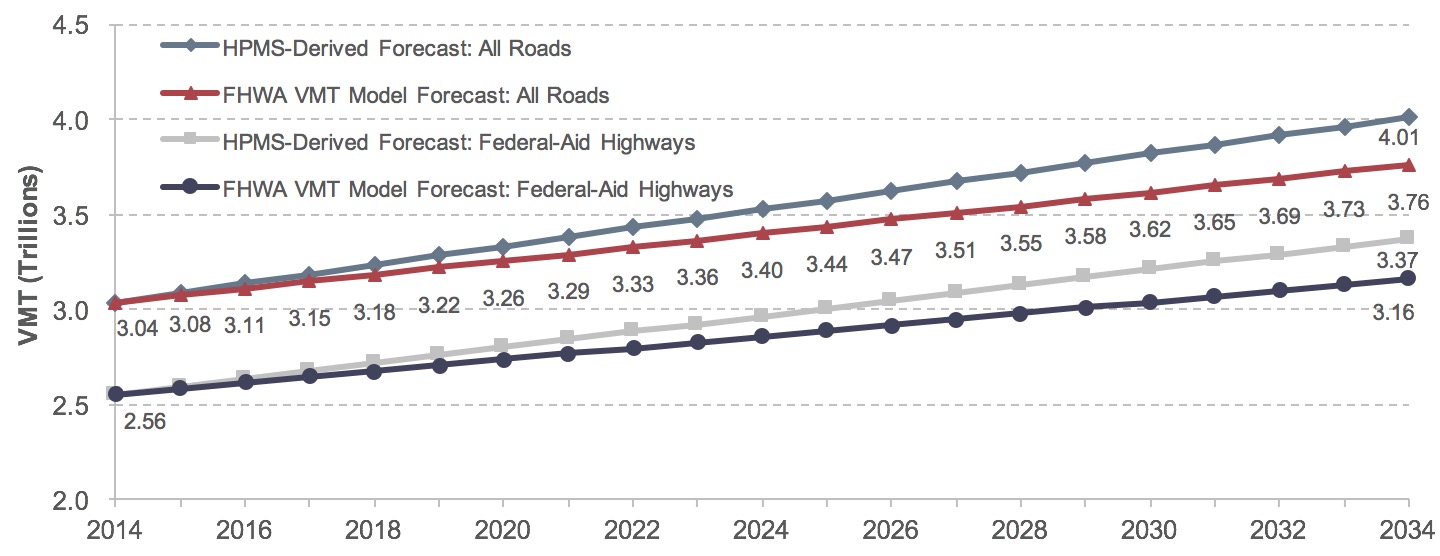
Sources: Highway Performance Monitoring System; FHWA Forecasts of Vehicle Miles Traveled (VMT), May 2017.
Exhibit 9-6: Impact of Alternative Travel Growth Forecasts on Highway Investment Scenario Average Annual Investment Levels
| Alternative Assumptions About Future Annual VMT Growth1 | Maintain Conditions and Performance Scenario | Improve Conditions and Performance Scenario | ||
|---|---|---|---|---|
| Billions of 2014 Dollars | Percent Change From Baseline | Billions of 2014 Dollars | Percent Change From Baseline | |
| Baseline2 (Tied to May 2017 Forecast—1.07% per year) | $102.4 | $135.7 | ||
| HERS-Derived Component | $59.5 | $73.2 | ||
| NBIAS-Derived Component | $12.9 | $22.7 | ||
| Other (Nonmodeled) Component | $30.0 | $39.8 | ||
| Lower (Tied to May 2016 Forecast—0.92% per year) | $100.9 | -1.4% | $131.1 | -3.4% |
| HERS-Derived Component | $58.5 | -1.7% | $70.3 | -4.0% |
| NBIAS-Derived Component | $12.9 | -0.2% | $22.4 | -1.4% |
| Other (Nonmodeled) Component | $29.6 | -1.4% | $38.4 | -3.4% |
| Higher (Tied to State Forecasts—HPMS at 1.40% per year; NBI at 1.45% per year) | $112.1 | 9.5% | $148.8 | 9.6% |
| HERS-Derived Component | $66.1 | 11.1% | $81.5 | 11.3% |
| NBIAS-Derived Component | $13.1 | 1.9% | $23.7 | 4.4% |
| Other (Nonmodeled) Component | $32.8 | 9.5% | $43.6 | 9.6% |
1 The VMT growth rates identified represent the forecasts entered into the HERS and NBIAS models. The travel demand elasticity features in HERS modify these forecasts in response to changes in highway user costs resulting from future highway investment.
2 The baseline levels shown correspond to the systemwide scenarios presented in Chapter 7. The investment levels shown are average annual values for the period from 2015 through 2034.
Sources: Highway Economic Requirements System and National Bridge Investment Analysis System.
Replacing the baseline traffic growth assumptions with the high-growth assumptions has much larger effects on the estimated investment requirements, consistent with the change in the annual growth rate (0.33 percent per year) being much larger. The resulting increase in the estimated investment requirement is 9.6 percent in the Improve Conditions and Performance scenarios and virtually the same in the Maintain Conditions and Performance scenario. The percentage effect is again considerably larger for the HERS component of the investment requirement than for the NBIAS component.
Key Takeaways
- Changes in Replacement Thresholds: TERM is very sensitive to changes in replacement thresholds. A 0.5 point change in the condition scale results in roughly ± 30 percent in replacement needs.
- Change in Capital Costs:
- SGR (no benefit-cost analysis test): The change in capital costs for preservation costs is comparable to the change in replacement investment costs.
- High- and Low-Growth scenarios (applies BCA test): a 25% increase in capital cost results in 18-25% increase in investment costs.
- Value of Time for Preservation Needs: Low sensitivity to variations in value of time. Doubling the value of time cost (from $12.80 to $25.60) increases investment costs by 5-6%.
- Discount Rate: Changes in the discount rate from 7% to 3% leads to an increase of 4% in investment levels.
Transit Sensitivity Analysis
This section examines the sensitivity of estimated transit investment needs, as produced by the Transit Economic Requirements Model (TERM), to variations in key inputs, including:
- asset replacement timing (condition threshold),
- capital costs,
- value of time, and
- discount rate.
The alternative projections presented in this chapter assess how the estimates of baseline investment needs for the State of Good Repair (SGR) benchmark and the Low-Growth and High-Growth scenarios discussed in Chapter 7 vary in response to changes in the assumed values of the input variables listed above. Note that, by definition, funding under the Sustain 2014 Expenditure scenario does not vary with changes in any input variable, and thus this scenario is not considered in this sensitivity analysis.
Changes in Asset Replacement Timing (Condition Threshold)
Each of the four investment scenarios examined in Chapter 7 assumes that assets are replaced at condition rating 2.50 as determined by TERM’s asset condition decay curves (in this context, 2.50 is referred to as the “replacement condition threshold”). TERM’s condition rating scale runs from 5.0 for assets in “excellent” condition through 1.0 for assets in “poor” condition. In practice, this assumption implies replacement of assets within a short period (e.g., roughly 1 to 5 years, depending on asset type) of their having attained their expected useful lives. Replacement at condition 2.50 can therefore be thought of as providing a replacement schedule that is both realistic and potentially conservative. This replacement schedule is realistic because, in practice, few assets are replaced exactly at their expected useful life value due to many factors, including the time to plan, fund, and procure asset replacement, and whether the assets are replaceable or not. A nonreplaceable asset is subjected only to maintenance activities, which generally accounts for a small share of its total replacement cost (see Box “How does TERM Handle Non-Replaceable Assets?” in Chapter 6). Its decay continues past the 2.50 replacement threshold. Examples of nonreplaceable assets include assets with long useful lives such as bridges, stations, tunnels, and other long-lived assets. It is a potentially conservative schedule because the needs estimates would be higher if all assets were to be replaced at precisely the end of their expected useful lives, and if nonreplaceable assets were replaceable.
Exhibit 9-7 shows the effect of varying the replacement condition threshold by increments of 0.25 on TERM’s projected asset preservation needs for the SGR benchmark and the Low-Growth and High-Growth scenarios. Note that selection of a higher replacement condition threshold results in assets being replaced while in better condition (i.e., at an earlier age). This, in turn, reduces the length of each asset’s service life, thus increasing the number of replacements over any given period of analysis and driving up scenario costs. Reducing the replacement condition threshold would have the opposite effect. As shown in Exhibit 9-7, each of these three scenarios shows significant changes to total estimated preservation needs from quarter-point changes in the replacement condition threshold. Relatively small changes in the replacement condition threshold frequently translate into significant changes in the expected useful life of some asset types; hence, small changes can also drive significant changes in replacement timing and replacement costs.
Exhibit 9-7: Impact of Alternative Replacement Condition Thresholds on Transit Preservation Investment Needs by Scenario (Excludes Expansion Impacts)
| Replacement Condition Thresholds | SGR Benchmark | Low Growth Scenario | High Growth Scenario | |||
|---|---|---|---|---|---|---|
| Billions of 2014 Dollars | Percent Change From Baseline | Billions of 2014 Dollars | Percent Change From Baseline | Billions of 2014 Dollars | Percent Change From Baseline | |
| Very Late Asset Replacement (2.00) | $12.1 | -29% | $11.5 | -34% | $11.5 | -34% |
| Replace Assets Later (2.25) | $14.8 | -13% | $14.0 | -19% | $14.1 | -19% |
| Baseline (2.50) | $17.0 | $17.4 | $17.5 | |||
| Replace Assets Earlier (2.75) | $21.7 | 27% | $20.4 | 18% | $20.6 | 18% |
| Very Early Asset Replacement (3.00) | $23.8 | 40% | $22.3 | 28% | $22.6 | 29% |
Source: Transit Economic Requirements Model.
Changes in Capital Costs
The asset costs used in TERM are based on actual prices paid by agencies for capital purchases as reported to the Federal Transit Administration (FTA) in the Transit Award Management System and in special surveys. Asset prices in the current version of TERM have been converted from the dollar-year replacement costs in which assets were reported to FTA by local agencies (which vary by agency and asset) to 2014 dollars using the RSMeans construction cost index. Given the uncertain nature of capital costs, a sensitivity analysis has been performed to examine the effect that higher capital costs would have on the dollar value of TERM’s baseline projected transit investment.
As Exhibit 9-8 shows, TERM projects that a 25-percent increase in capital costs (i.e., beyond the 2014 level used for this C&P Report) would be fully reflected in the SGR benchmark, but only partially realized under the Low-Growth or High-Growth scenarios. This difference in sensitivity results is driven by the fact that investments are not subject to TERM’s benefit-cost test in computing the SGR benchmark (i.e., increasing costs have no consequences), whereas the two cost-constrained scenarios do employ this test. Hence, for the Low-Growth or High-Growth scenarios, any increase in capital costs (without a similar increase in the value of transit benefits) results in lower benefit-cost ratios and the failure of some investments to pass this test. Therefore, for these latter two scenarios, a 25-percent increase in capital costs would yield a roughly 18- to 20-percent increase in needs that pass TERM’s benefit-cost test.
Exhibit 9-8: Impact of an Increase in Capital Costs on Transit Investment Estimates by Scenario
| Capital Cost Increases | SGR Benchmark | Low Growth Scenario | High Growth Scenario | |||
|---|---|---|---|---|---|---|
| Billions of 2014 Dollars | Percent Change From Baseline | Billions of 2014 Dollars | Percent Change From Baseline | Billions of 2014 Dollars | Percent Change From Baseline | |
| Baseline (No Change) | $17.1 | $23.4 | $25.5 | |||
| Increase Costs by 25% | $21.2 | 24% | $28.1 | 20% | $30.3 | 18% |
Source: Transit Economic Requirements Model.
Changes in the Value of Time
The most significant source of transit investment benefits, as assessed by TERM’s benefit-cost analysis, is the net cost savings to users of transit services, a key component of which is the value of travel time savings. Therefore, the per-hour value of travel time for transit riders is a key model input and a key driver of total investment benefits for those scenarios that use TERM’s benefit-cost test. Readers interested in learning more about the measurement and use of the value of time for the BCAs performed by TERM, the Highway Economic Requirements System (HERS), and the National Bridge Investment Analysis System (NBIAS) should refer to the related discussion presented earlier in the highway section of this chapter.
For this C&P Report, the Low-Growth and High-Growth scenarios are the only scenarios with investment needs estimates that are sensitive to changes in the benefit-cost ratio. (Note that the Sustain 2014 Spending scenario uses TERM’s estimated benefit-cost ratios to allocate fixed levels of funding to preferred investments, while the computation of the SGR benchmark does not.)
Exhibit 9-9 shows the effect of varying the value of time on the needs estimates of the Low-Growth and High-Growth scenarios. The baseline value of time for transit users in 2014 was $12.80 per hour, based on DOT guidance. TERM applies this amount to all in-vehicle travel, but then doubles it to $25.60 per hour when accounting for out-of-vehicle travel time, including time spent waiting at transit stops and stations (also consistent with DOT guidance).
Exhibit 9-9: Impact of Alternative Value of Time Rates on Transit Investment Estimates by Scenario
| Changes in Value of Time | Low Growth Scenario | High Growth Scenario | ||
|---|---|---|---|---|
| Billions of 2014 Dollars | Percent Change From Baseline | Billions of 2014 Dollars | Percent Change From Baseline | |
| Reduce by 50% ($6.4) | $21.0 | -10% | $22.2 | -13% |
| Baseline ($12.8) | $23.4 | $25.5 | ||
| Increase by 100% ($25.6) | $24.5 | 5% | $27.1 | 6% |
Source: Transit Economic Requirements Model.
Given that value of time is a key driver of total investment benefits, doubling or halving this variable leads to changes in investment ranging from an increase of roughly 5 percent to a decrease of nearly 10 percent. The High-Growth scenario appears to be more sensitive to the value of time than the Low-Growth scenario. This is because the High-Growth scenario is associated with higher investment levels than is the Low-Growth scenario, so any changes in the value of time will be magnified accordingly.
Changes to the Discount Rate
TERM’s benefit-cost module uses a discount rate of 7.0 percent, in accordance with guidance provided in OMB Circular A-94. Readers interested in learning more about the selection and use of discount rates for the BCAs performed by TERM, HERS, and NBIAS should refer to the related discussion presented earlier in the highway section of this chapter. For this sensitivity analysis, and for consistency with the discussion above on HERS and NBIAS discount rate sensitivity, TERM’s needs estimates for the Low-Growth and High-Growth scenarios were re-estimated using a 3-percent discount rate. The results of this analysis, presented in Exhibit 9-10, show that this lower discount rate leads to a range in total investment needs (or changes in the proportion of needs passing TERM’s benefit-cost test) amounting to between a 4- and 5.6-percent increase.
Exhibit 9-10: Impact of Alternative Discount Rates on Transit Investment Estimates by Scenario
| Discount Rates | Low Growth Scenario | High Growth Scenario | ||
|---|---|---|---|---|
| Billions of 2014 Dollars | Percent Change From Baseline | Billions of 2014 Dollars | Percent Change From Baseline | |
| 7.0% (Baseline) | $23.4 | $25.5 | ||
| 3.0% | $24.3 | 4% | $27.0 | 6% |
Source: Transit Economic Requirements Model.
Under this sensitivity test, investment needs are usually higher for the lower (3 percent) discount rate compared with the higher base rate (7 percent). This means that use of the lower rate allows more investments to pass TERM’s benefit-cost test. This situation is primarily the result of differences in the timing of the flows of benefits versus costs for the underlying scenario. Specifically, this test uses a fully (financially) unconstrained scenario that completely eliminates the large investment backlog at the start of the period of analysis and then invests incrementally as needed at a much lower rate to maintain this “state of good repair” for the remaining 20 years of analysis. In contrast, investment benefits tend to be more evenly distributed throughout the 20-year period of analysis. So, with a high proportion of costs concentrated very early in the period of analysis and evenly distributed benefits, the ratio of discounted benefits to discounted costs tends to decline as the discount rate increases.