

Chapter 10: Impacts of Investment
- Impacts of Highway Investment
- HERS, NBIAS, and Nonmodeled Inputs to the Improve Conditions and Performance Scenario
- Impacts of Federal-aid Highway Investments Modeled by HERS
- Selection of Investment Levels for Analysis
- Investment Levels and BCRs by Funding Period
- Impact of Future Investment on Highway Pavement Ride Quality
- Impact of Future Investment on Highway Operational Performance
- Impact of Future Investment on Highway User Costs
- Impact on Vehicle Operating Costs
- Impact of Future Investment on Future VMT
- Impacts of NHS Investments Modeled by HERS
- Impacts of Interstate System Investments Modeled by HERS
- Impacts of Systemwide Investments Modeled by NBIAS
- Impacts of Federal-aid Highway Investments Modeled by NBIAS
- Impacts of NHS Investments Modeled by NBIAS
- Impacts of Interstate System Investments Modeled by NBIAS
- Impacts of Transit Investment
- Impacts of Systemwide Investments Modeled by TERM
- Impact of Preservation Investments on Transit Backlog and Conditions
- Impact of Expansion Investments on Transit Ridership

Key Takeaways
- Due to the impact of travel demand elasticity procedures, the HERS model predicts an annual percentage change in VMT on Federal-aid Highways of 1.13 to 1.22 percent for the range of investment levels analyzed compared with the 1.07 percent assumed if user costs remain unchanged in the future.
- HERS finds it to be cost-beneficial to reduce the percentage of travel on pavements with poor ride quality, but not necessarily to reduce average pavement roughness. For the NHS and Interstate highways, average IRI would get worse even at the Improve Conditions and Performance scenario level.
- Unlike for bridges overall, or bridges on Federal-aid highways, NBIAS finds that sustaining spending at 2014 levels for NHS bridges and Interstate bridges would be insufficient to keep the deck area-weighted share of bridges in poor conditions from rising over time.
Impacts of Highway Investment
The analyses presented in this section use a common set of assumptions to derive relationships between alternative levels of future highway capital investment and various measures of future highway and bridge conditions and performance. A subsequent section in this chapter provides comparable information for different types and levels of potential future transit investments.
This section examines the types of investment within the scopes of the Highway Economic Requirements System (HERS) and the National Bridge Investment Analysis System (NBIAS) and provides more context for the capital investment scenarios for highways presented in Chapter 7. The accuracy of projections for highway investments in this chapter depends on the validity of the technical assumptions underlying the analysis, some of which are explored in the sensitivity analysis in Chapter 9. The analyses presented in this section make no explicit assumptions regarding how future investment in highways could be funded.
HERS, NBIAS, and Nonmodeled Inputs to the Improve Conditions and Performance Scenario
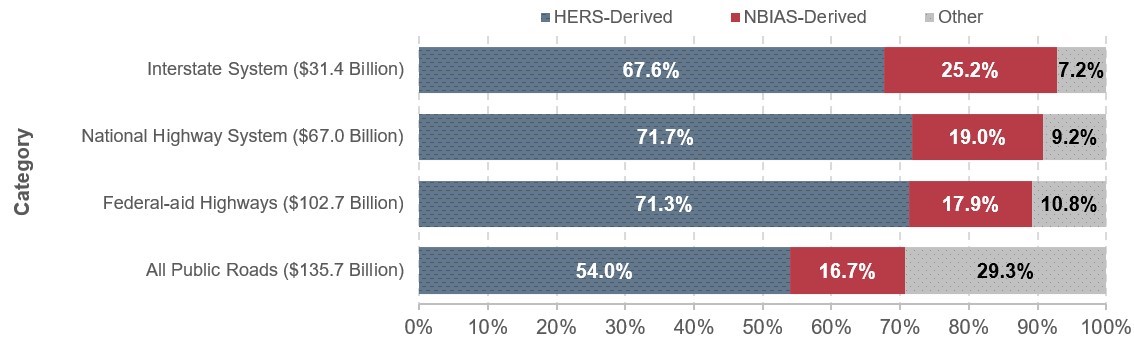
Exhibit 10-1 illustrates the derivation of the Improve Conditions and Performance scenario presented in Chapter 7. Of the $135.7 billion average annual investment level for all public roads under this scenario, 16.7 percent was derived from NBIAS (corresponding to the $22.7 billion identified as “System Rehabilitation – Bridge” in the “All Public Roads” row) and 54.0 percent was derived from HERS (corresponding to the $49.0 billion and $24.2 billion identified as “System Rehabilitation – Highways” and “System Expansion,” respectively, in the “Federal-aid Highways” row). The remaining 29.3 percent was nonmodeled; this corresponds to the $18.3 billion identified as “System Enhancement” in the “All Public Roads” row plus the difference between the amounts shown in the “All Public Roads” and the “Federal-aid Highway” rows for “System Rehabilitation – Highways” ($16.7 billion, computed as $65.7 billion minus $49.0 billion) and “System Expansion” ($4.9 billion, computed as $29.1 billion minus $24.2 billion). Each of the nonmodeled input values was computed using scaling procedures so that its share of the total scenario investment level would match its share of actual 2014 spending.
Exhibit 10-1 also identifies the average annual investment levels resulting from applying the Improve Conditions and Performance scenario criteria to various system subsets including the Interstate Highway System ($31.4 billion), the National Highway System (NHS) ($67.0 billion, including the amount directed to Interstate highways), and Federal-aid Highways ($102.7 billion, including the amount directed to the NHS). The modeled share of investment on these systems is higher than for all public roads because HERS and NBIAS fully cover system rehabilitation and system expansion investments on these types of highways, and only system enhancement investment is outside the scope of the two models.
The average annual investment level for the Federal-aid highways is 71.3 percent HERS-derived, 17.9 percent NBIAS-derived, and 10.8 percent nonmodeled. The average annual investment level for the Federal-aid highways is 71.3 percent HERS-derived, 17.9 percent NBIAS-derived, and 10.8 percent nonmodeled. The share of spending by source of estimate for the NHS is similar to that for Federal-aid highways, but the Interstate distribution is somewhat different with 67.6 percent HERS-derived, 25.2 percent NBIAS-derived, and 7.2 percent nonmodeled.
Exhibit 10-1: Improve Conditions and Performance Scenario for 2015 Through 2034: Distribution by System, by Source of Estimate, and by Capital Improvement Type
| System Component | System Rehabilitation | System Expansion | System Enhancement | Total | Percent of Total | ||
|---|---|---|---|---|---|---|---|
| Highway | Bridge | Total | |||||
| Average Annual Investment in Billions of 2014 Dollars | |||||||
| Interstate Highway System | $11.9* | $7.9^ | $19.9 | $9.3* | $2.3 | $31.4 | 23.2% |
| National Highway System | $29.6* | $12.8^ | $42.3 | $18.5* | $6.2 | $67.0 | 49.4% |
| Federal-aid Highways | $49.0* | $18.4^ | $67.4 | $24.2* | $11.1 | $102.7 | 75.7% |
| All Public Roads | $65.7 | $22.7^ | $88.4 | $29.1 | $18.3 | $135.7 | 100.0% |
Note: The “NBIAS-Derived” share includes all outlays (values shown as red^ in the table) classified as “System Rehabilitation: Bridge.” The “HERS-Derived” share includes most outlays (values shown as blue* in the table) classified as “System Rehabilitation: Highway” and “System Expansion” except for the portions spent off of Federal-aid Highways, which are classified as “Other.” The “Other” category also includes all outlays classified as “System Enhancement.”
Sources: Highway Economic Requirements System and National Bridge Investment Analysis System.
The top row in each table in Exhibits 10-2 through 10-18 corresponds to values presented in Exhibit 10-1 as HERS-derived or NBIAS-derived inputs to the Improve Conditions and Performance scenario presented in Chapter 7.
How were the investment levels presented in Exhibits 10-2 to 10-18 selected?
The particular investment levels shown in each exhibit were selected from the results of a much larger number of model simulations. All are meant to be illustrative; some were chosen to align with the scenarios presented in Chapter 7, but others were simply chosen to show a relatively even distribution of data points for the charts. There is no special significance to the lowest investment level shown in each table.
Most of the HERS and NBIAS analyses presented in this chapter assume a fixed amount of spending in constant dollars in each of the 20 years of the analysis period. However, the highest levels shown (the one or more shown above the bold horizontal line in the tables) are based on model runs constrained by a benefit-cost ratio.
Impacts of Federal-aid Highway Investments Modeled by HERS
The HERS analysis for this edition of the C&P Report starts with an evaluation of the state of Federal-aid highways in 2014—the base year. In the Introduction to Part II, Exhibit II-1 shows that capital spending on the types of improvements modeled in HERS for these highways in the base year was $60.2 billion (total highway capital spending was $105.4 billion). The analysis continues by considering the potential impacts on system performance of raising or lowering the amount of investment within the scope of HERS over 20 years. Spending in any year is measured in constant 2014 (real) dollars, rather than nominal dollars.
Selection of Investment Levels for Analysis
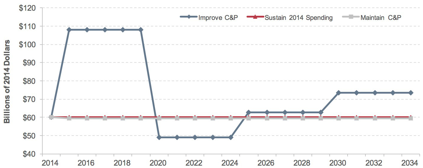
Exhibit 10-2 introduces the nine investment levels presented in the next several exhibits to illuminate the relationship between the levels of investment modeled in HERS and the future conditions and performance of Federal-aid highways. The “Improve C&P” reference in the top row of Exhibit 10-2 signifies that this level of investment feeds into the Improve Conditions and Performance scenario in Chapter 7, which is defined by attaining a minimum benefit-cost ratio (BCR) of 1.0 in each year over the 20-year analysis period. The remaining eight runs are funding-constrained, for which HERS ranks potential projects in order of BCR and implements them until the funding constraint is reached.
One funding level shown in Exhibit 10-2 represents the spending level designed to match a specific level of performance in 2034; a spending level of $59.5 billion is projected to be adequate to allow average pavement roughness as measured by the International Roughness Index (IRI) in 2034 to match the level in 2014 (see discussion of IRI in Chapter 6) and for average delay to be at least as low in 2034 as it was in 2014. The “Maintain C&P” reference in Exhibit 10-2 signifies that this level of investment feeds into the Maintain Conditions and Performance scenario presented in Chapter 7.
The “2014 Spending” reference in Exhibit 10-2 signifies that this level of spending feeds into the Sustain 2014 Spending scenario presented in Chapter 7. The remaining six of the nine funding levels shown in Exhibit 10-2 represent roughly $4.0 billion increases from $49.0 billion to $73.2 billion (Improve C&P).
The portion of each investment level that HERS directs to system rehabilitation versus system expansion is important, as these types of investments have varying degrees of influence on different performance measures. Investment in system rehabilitation (ranging from $34.3 billion to $49.0 billion across reported investment levels) tends to have a stronger influence on physical condition measures such as pavement ride quality. Investment in system expansion (ranging from $14.7 billion to $24.2 billion across reported investment levels) has a more pronounced impact on operational performance measures such as delay.
Investment Levels and BCRs by Funding Period
Exhibit 10-2 illustrates how the nine alternative funding levels for Federal-aid highways that were selected for further analysis in this chapter would translate into cumulative spending in 5-year intervals (corresponding to 5-year analysis periods used in HERS).
As shown in Exhibit 10-2, achieving a minimum BCR of 1.0 is estimated to require $1.465 trillion over the 20-year analysis period. This would necessitate an increase in spending of $262 billion over the analysis period relative to the $1.203 trillion 20-year cost of a scenario in which 2014 spending levels were sustained from 2014 through 2034.
Exhibit 10-2: HERS Annual Investment Levels Analyzed for Federal-aid Highways
| Spending Modeled in HERS (Billions of 2014 Dollars) | Link to Chapter 7 Scenario | ||||||||
|---|---|---|---|---|---|---|---|---|---|
| Average Annual Over 20 Years | Cumulative | ||||||||
| Total HERS Spending | System Rehabilitation Spending1 | System Expansions Spending1 | 5-Year 2013 Through 2017 | 5-Year 2018 Through 2022 | 5-Year 2023 Through 2027 | 5-Year 2028 Through 2032 | 20-Year 2013 Through 2032 | ||
| $73.2 | $49.0 | $24.2 | $540 | $245 | $313 | $367 | $1,465 | Improve C&P | |
| $68.9 | $46.4 | $22.5 | $344 | $345 | $344 | $345 | $1,378 | ||
| $65.0 | $44.1 | $20.9 | $325 | $325 | $325 | $325 | $1,300 | ||
| $61.0 | $41.9 | $19.1 | $305 | $305 | $305 | $305 | $1,220 | ||
| $60.2 | $41.5 | $18.7 | $301 | $301 | $301 | $301 | $1,203 | 2014 Spending | |
| $59.5 | $41.0 | $18.5 | $297 | $297 | $297 | $297 | $1,190 | Maintain C&P | |
| $57.0 | $39.4 | $17.6 | $285 | $285 | $285 | $285 | $1,140 | ||
| $53.0 | $37.0 | $16.0 | $265 | $265 | $265 | $265 | $1,060 | ||
| $49.0 | $34.3 | $14.7 | $245 | $245 | $245 | $245 | $980 | ||
1 HERS splits its available budget between system rehabilitation and system expansion based on the mix of spending it finds to be most cost-beneficial, which varies by funding level.
Source: Highway Economic Requirements System.
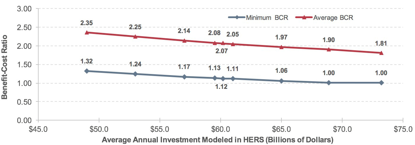
Exhibit 10-3 illustrates the marginal BCRs (i.e., the lowest BCR among the improvements selected within a funding period) associated with the nine alternative funding levels. Exhibit 10-3 also provides the minimum BCRs across all funding periods (which is identical to the lowest marginal BCR) and the average BCRs across all funding periods (i.e., the total level of benefits of all improvements divided by the total cost of all improvements). The marginal BCRs for the top row are all 1.00, as this analysis allowed spending levels to vary by funding period specifically to result in this outcome.
Exhibit 10-3: Minimum and Average Benefit-Cost Ratios (BCRs) for Different Possible Funding Levels on Federal-aid Highways
| HERS-Modeled Investment on Federal-Aid Highways Average Annual Investment (Billions of 2014 Dollars) |
Benefit-Cost Ratios1 | Link to Chapter 7 Scenario | |||||
|---|---|---|---|---|---|---|---|
| Average BCR 20-Year 2015 Through 2034 | Marginal BCR2 | Minimum BCR 20-Year 2015 Through 2034 | |||||
| 5-Year 2015 Through 2019 | 5-Year 2020 Through 2024 | 5-Year 2025 Through 2029 | 5-Year 2030 Through 2034 | ||||
| $73.2 | 1.81 | 1.00 | 1.00 | 1.00 | 1.00 | 1.00 | Improve C&P |
| $68.9 | 1.90 | 1.36 | 1.08 | 1.00 | 1.01 | 1.00 | |
| $65.0 | 1.97 | 1.41 | 1.13 | 1.06 | 1.06 | 1.06 | |
| $61.0 | 2.05 | 1.46 | 1.18 | 1.11 | 1.11 | 1.11 | |
| $60.2 | 2.07 | 1.47 | 1.19 | 1.12 | 1.12 | 1.12 | 2014 Spending |
| $59.5 | 2.08 | 1.48 | 1.20 | 1.13 | 1.13 | 1.13 | Maintain C&P |
| $57.0 | 2.14 | 1.52 | 1.24 | 1.17 | 1.18 | 1.17 | |
| $53.0 | 2.25 | 1.59 | 1.31 | 1.24 | 1.25 | 1.24 | |
| $49.0 | 2.35 | 1.68 | 1.38 | 1.32 | 1.33 | 1.32 | |
1 As HERS ranks potential improvements by their estimated BCRs and assumes that the improvements with the highest BCRs will be implemented first (up until the point where the available budget specified is exhausted), the minimum and average BCRs will naturally tend to decline as the level of investment analyzed rises.
2 The marginal BCR represents the lowest benefit-cost ratio for any project implemented during the period identified at the level of funding shown. The minimum BCRs, indicated by bold font, are the smallest of the marginal BCRs across the funding periods.
Source: Highway Economic Requirements System.
For the analyses assuming fixed levels of spending each year, the marginal BCR is highest in the first funding period and then declines over time, reflecting the tendency in HERS to implement the most worthwhile improvements first. However, by the fourth funding period the marginal BCRs begin to creep back up slightly (not evident in all rows due to rounding), so that the minimum BCR over the entire 20-year analysis period equals the marginal BCR in the third 5-year period. This pattern reflects the impacts of funding constraints; the relative scarcity of funding toward the end of the analysis period is inadequate to keep pace with newly emerging needs, limiting the range of needs that can be addressed.
Further evident in Exhibit 10-3 is the inverse relationship between the minimum BCR and the level of investment. At any given level of average annual investment, the average BCR always exceeds the marginal BCR. For example, at the highest level of investment considered, an average annual investment level of $73.2 billion, the average BCR of 1.81 exceeds the minimum BCR of 1.00.
Impact of Future Investment on Highway Pavement Ride Quality
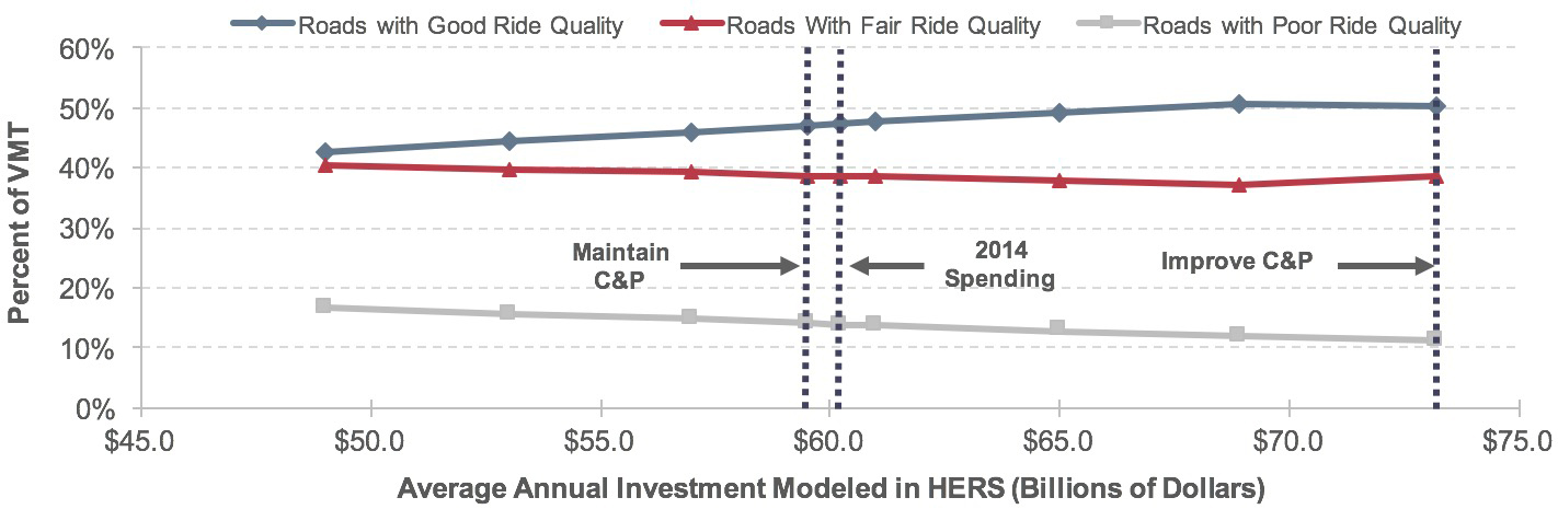
For all investment levels above Maintain C&P presented in Exhibit 10-4, pavements on Federal-aid highways are projected to be smoother on average in 2034 than in 2014. For the $59.5 billion average annual HERS investment level associated with the Maintain C&P scenario, pavements on Federal-aid highways are projected to be as smooth on average in 2034 as they were in 2014, while for the lower investment levels ($57.0 billion and lower) Federal-aid highways are projected to have higher average IRI in 2034 than in 2014. VMT-weighted average IRI decreases by up to 13.2 percent across alternatives (from 124.0 to 110.8), from an investment level that increases average IRI by 5.6 percent to the top-line investment level that reduces average IRI by 5.6 percent.
Exhibit 10-4 also shows the HERS projections for the percentage of travel occurring on pavements with ride quality that would be rated “good,” “fair,” and “poor” based on the IRI thresholds described in Chapter 6. Under all circumstances represented in the exhibit, the 2034 projection for the percentage of travel occurring on pavements with “poor” ride quality is lower than the 17.3 percent that occurred in 2014, as the model identifies significant user benefits that can be obtained by addressing pavement deficiencies. Among the rows depicting analyses with fixed annual investment levels, the improvement in the share of travel on pavements with “good” ride quality increases roughly linearly with spending, while the share of travel on roads with “fair” ride quality decrease roughly linearly with spending.
The projections for the percentage of VMT with “good” ride quality for 2034 range from 50.7 percent at the second-highest level of average annual investment modeled (an average annual investment for system rehabilitation of $46.4 billion) to 42.6 percent at the lowest level of investment (an average annual investment for system rehabilitation of $34.3 billion).
Relative to the second row, the top row of Exhibit 10-4 shows a slightly lower percentage of VMT on pavements with good ride quality (50.2 percent versus 50.7 percent) and a slightly higher share of VMT on pavements with fair ride quality (38.7 percent versus 37.2 percent). This result is an artifact of the relatively front-loaded investment pattern associated with the minimum-BCR-driven analysis reflected in the top row: some of the pavements improved in the surge of investment in the first funding period would have declined to fair condition by 2034, but would not yet warrant additional corrective actions. Looking over the full 20-year analysis period rather than just a single point in time (2034), the average percentage of pavements with good ride quality would be highest for the average annual investment level for system rehabilitation of $49.0 billion identified in the top row.
As noted in Chapter 6, the IRI threshold of 170 used to identify fair ride quality was originally set to measure performance on the NHS and may not be fully applicable to non-NHS routes, which tend to have lower travel volumes and speeds. This helps to explain why the percentage of VMT on roads with poor ride quality falls no lower than 11.2 percent, even when all cost-beneficial improvements are implemented. In some cases, the benefits of potential pavement improvements may not exceed their costs until the IRI has increased to a level well higher than the threshold of 170.
Exhibit 10-4: Projected Impact of Alternative Investment Levels on 2034 Pavement Ride Quality Indicators for Federal-aid Highways
| HERS-Modeled Capital Investment Average Annual Spending (Billions of 2014 Dollars) |
Projected 2034 Condition Measures on Federal-aid Highways1,2 | Link to Chapter 7 Scenario | |||||
|---|---|---|---|---|---|---|---|
| Percent of VMT on Roads With Ride Quality of: | Average IRI (VMT-Weighted) | ||||||
| Total | System Rehabilitation2 |
Good (IRI>95)3 | Fair (IRI 95 to 170) | Poor (IRI>170)3 | Inches Per Mile | Change Relative to Base Year | |
| $73.2 | $49.0 | 50.2% | 38.7% | 11.2% | 110.8 | -5.6% | Improve C&P |
| $68.9 | $46.4 | 50.7% | 37.2% | 12.1% | 112.4 | -4.3% | |
| $65.0 | $44.1 | 49.3% | 37.8% | 12.9% | 114.3 | -2.6% | |
| $61.0 | $41.9 | 47.6% | 38.5% | 13.8% | 116.6 | -0.7% | |
| $60.2 | $41.5 | 47.5% | 38.5% | 13.9% | 117.0 | -0.3% | 2014 Spending |
| $59.5 | $41.0 | 47.2% | 38.8% | 14.1% | 117.4 | 0.0% | Maintain C&P |
| $57.0 | $39.4 | 45.9% | 39.3% | 14.8% | 119.0 | 1.4% | |
| $53.0 | $37.0 | 44.4% | 39.8% | 15.8% | 121.4 | 3.4% | |
| $49.0 | $34.3 | 42.6% | 40.5% | 16.9% | 124.0 | 5.6% | |
| Base Year Values: | 47.0% | 35.7% | 17.3% | 117.4 | |||
1 The HERS model relies on information from the HPMS sample section database, which is limited to those portions of the road network that are generally eligible for Federal funding (i.e., “Federal-aid highways”) and excludes roads classified as rural minor collectors, rural local, and urban local.
2 The system rehabilitation component of HERS-modeled spending would likely have a greater impact on the performance indicators in this exhibit than would the system expansion component that is also reflected in the total.
3 As discussed in Chapter 6, IRI values of 95 through 170 inches per mile are classified as “fair,” lower IRI values are classified as “good,” and higher IRI values are classified as “poor.”
Source: Highway Economic Requirements System.
Impact of Future Investment on Highway Operational Performance
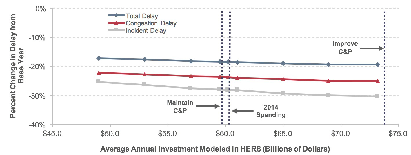
Exhibit 10-5 shows the HERS projections for the impact of investment levels on average speed and traveler delay. Exhibit 10-5 splits out the portion of the investment that HERS allocates for system expansion (such as widening existing highways or building new routes in existing corridors), which tends to reduce congestion delay more than spending on system rehabilitation. The tabular portion of the exhibit shows that the levels of system expansion analyzed range from an average annual investment of $14.7 billion (which feeds the Maintain Conditions and Performance scenario in Chapter 7) to an average annual investment of $24.2 billion (which feeds the Improve Conditions and Performance scenario in Chapter 7). The graph is plotted based on total average annual investment modeled in HERS, including spending on both system rehabilitation and system expansion.
Exhibit 10-5: Projected Impact of Alternative Investment Levels on 2034 Highway Travel Delay and Speed on Federal-aid Highways
| HERS-Modeled Capital Investment Average Annual Spending (Billions of 2014 Dollars) |
Projected 2034 Performance Measures on Federal-aid Highways |
Link to Chapter 7 Scenario | |||||
|---|---|---|---|---|---|---|---|
| Average Speed in 2034 (mph) | Annual Hours of Delay per Vehicle2 | Percent Change Relative to Baseline |
|||||
| Total | System Expansion1 |
Total Delay per VMT | Congestion Delay per VMT | Incident Delay per VMT | |||
| $73.2 | $24.2 | 45.2 | 37.8 | -19.3% | -24.9% | -30.3% | Improve C&P |
| $68.9 | $22.5 | 45.2 | 37.8 | -19.4% | -24.9% | -30.0% | |
| $65.0 | $20.9 | 45.2 | 38.0 | -19.0% | -24.4% | -29.3% | |
| $61.0 | $19.1 | 45.1 | 38.2 | -18.5% | -23.9% | -28.1% | |
| $60.2 | $18.7 | 45.1 | 38.2 | -18.5% | -23.7% | -28.1% | 2014 Spending |
| $59.5 | $18.5 | 45.1 | 38.3 | -18.4% | -23.6% | -28.0% | Maintain C&P |
| $57.0 | $17.6 | 45.1 | 38.4 | -18.2% | -23.3% | -27.6% | |
| $53.0 | $16.0 | 45.0 | 38.6 | -17.6% | -22.7% | -26.3% | |
| $49.0 | $14.7 | 45.0 | 38.8 | -17.2% | -22.1% | -25.4% | |
| Base Year Values: | 43.1 | 46.9 | |||||
1 The system expansion component of HERS-modeled spending would likely have a greater impact on the performance indicators in this exhibit than would the system rehabilitation component that is also reflected in the total.
2 The values shown were computed by multiplying HERS estimates of average delay per VMT by 11,742, the average VMT per registered vehicle in 2014. HERS does not forecast changes in VMT per vehicle over time. The HERS delay figures include delay attributable to stop signs and signals as well as delay resulting from congestion and incidents.
Source: Highway Economic Requirements System; Highway Statistics 2015, Table VM-1.
The results in Exhibit 10-5 reveal investment within the scope of HERS to be a potent instrument for reducing congestion delay. HERS projects congestion delay to decrease by between 22.1 percent and 24.9 percent between 2014 and 2034.
Across all scenarios presented in Exhibit 10-5, annual delay per vehicle in 2034 is lower than the 2014 level (46.9 hours), with reductions in delay ranging narrowly from 8.1 hours in the lowest level of investment analyzed to 9.1 hours in the highest. The projected increases in average vehicle speed are similarly narrow, ranging from 45.0 miles per hour to 45.2 miles per hour, compared with the 2014 level of 43.1 miles per hour.
Some traffic basics are important to keep in mind when interpreting these results. In addition to congestion and incident delay, some delay inevitably results from traffic control devices. For this reason, and because traffic congestion occurs only at certain places and times, Exhibit 10-5 shows the variation in investment levels as having less impact on projections for total delay and average speed than on the projections for congestion and incident delay. In addition, although the impacts of additional investment on average speed are proportionally small, these impacts apply to a vast amount of travel; hence, the associated savings in user cost are not necessarily small relative to the cost of the investment.
Impact of Future Investment on Highway User Costs
In HERS, the benefits from highway improvements are measured as reductions in highway user costs, agency costs, and societal costs of vehicle emissions. In measuring the highway user costs, the model includes the costs of travel time, vehicle operation, and crashes.
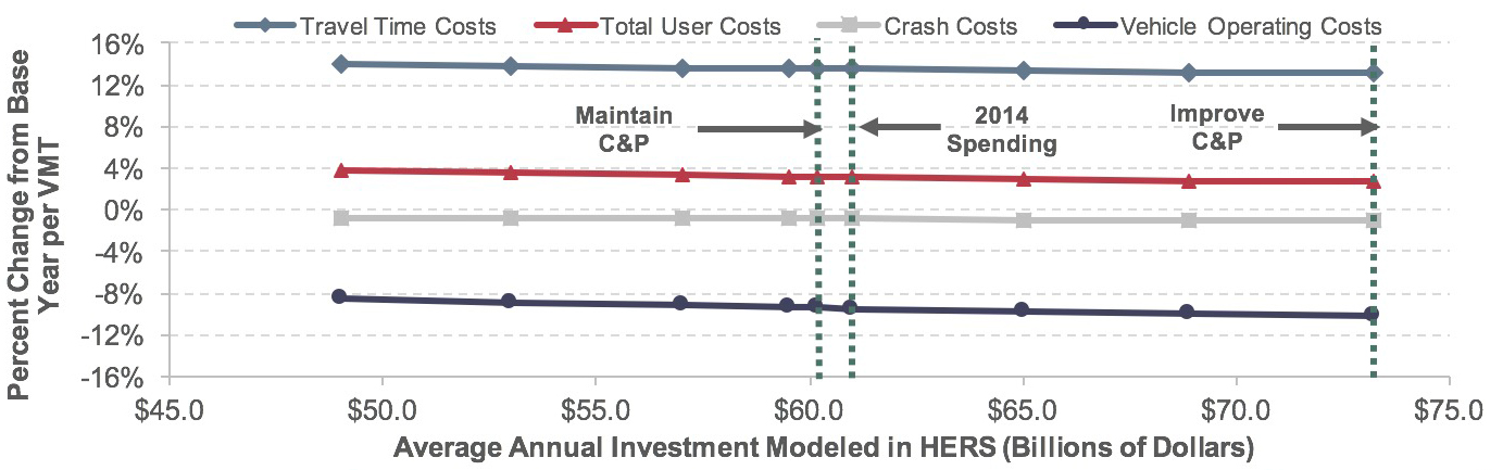
Exhibit 10-6 shows the projected changes from 2014 in average user cost of travel on Federal-aid highways by cost component. For Federal-aid highways, HERS estimates that user costs—the costs of travel time, vehicle operation, and crashes—averaged $1.262 per mile traveled in 2014.
Average user cost per VMT is projected to increase from the 2014 values by 3.7 percent at the lowest level of spending ($49.0 billion) to 2.7 percent at the highest level of spending ($73.2 billion, which feeds the Improve Conditions and Performance scenario in Chapter 7). The cost of crashes is the user cost component with the lowest absolute sensitivity to the assumed level of highway investment. Crash costs in 2034 are projected to be between 0.7 percent and 1.0 percent lower than in 2014.
What are the monetized national-level impacts implied by the changes in average user costs projected by HERS?
Exhibit 10-6 presents measures of average user costs per VMT, rather than projections of aggregate, national-level user costs. User costs comprise the costs of travel time, vehicle operation (fuel, maintenance & repairs, etc.), and crashes for all vehicle occupants (highway “users”). To identify monetized impacts of changes in investment levels on national-level user costs, national VMT in 2034 can be multiplied by differences in average user costs across investment levels. At the highest level of investment (an annual average of $73.2 billion), average total user costs are projected to be $1.296 per VMT. Average total user costs at the highest level of investment represent decreases in average total user costs of $0.006 per VMT when spending is held at the base-year level ($60.2 billion per year) and $0.013 per VMT at the lowest level of investment (an annual average of $49.0 billion).
Investing at the highest level is projected to result in a decrease in total user costs in 2034 of $44.2 billion relative to the lowest level of investment ($49.0 billion per year) analyzed. Investing at the highest level is projected to result in a decrease in total user costs in 2034 of $20.4 billion relative to investing at the base-year level.
Approximately half the projected national-level impacts on average user costs can be attributed to impacts on vehicle operating costs. At the highest investment level, average vehicle operating costs per VMT in 2034 are projected to be $0.008 lower than under the lowest investment level and $0.004 lower than when spending is held at the base-year level. Investing at the highest level is projected to result in a decrease in total vehicle operating costs in 2034 of $25.3 billion relative to the lowest level of investment, based on projected VMT for the lowest investment level in 2034. Investing at the highest level is projected to result in a decrease in total vehicle operating costs in 2034 of $12.7 billion relative to investing at the base-year level, based on projected VMT for the lowest investment level in 2034.
The levels of spending in each scenario are limited to the types of improvements that HERS evaluates, which are basically system rehabilitation and expansion. Because HPMS lacks detailed information on the current location and characteristics of safety-related features (e.g., guardrail, rumble strips, roundabouts, yellow change intervals at signals), safety-focused investments are not evaluated. Thus, the findings presented in Exhibit 10-6 establish nothing about how such investments affect highway safety.
Crash costs also form the smallest of the three components of highway user costs. For 2014 travel on Federal-aid highways, HERS estimates the breakdown by cost component for each spending level. The average across spending levels for each share of user costs are crash cost, 12.7 percent; travel time cost, 54.7 percent, and vehicle operating cost, 32.4 percent. Research underway to update the vehicle operating cost equations in HERS (see Appendix A) could somewhat alter the split among these costs in future reports, but crash costs will likely remain a relatively small component. Although highway trips always consume traveler time and resources for vehicle operation, only a small fraction involve crashes. In addition, many crashes involve only damage to property with no injuries, particularly on urban highways.
Exhibit 10-6: Projected Impact of Alternative Investment Levels on 2034 Average Total User Costs on Federal-aid Highways
| HERS-Modeled Investment On Federal-aid Highways Average Annual Investment (Billions of 2014 Dollars) | Projected 2034 Performance Measures on Federal-aid Highways | Link to Chapter 7 Scenario | ||||
|---|---|---|---|---|---|---|
| Average Total User Costs ($/VMT) | Percent Change Relative to Baseline Average per VMT | |||||
| Total User Costs | Travel Time Costs | Vehicle Operating Costs | Crash Costs | |||
| $73.2 | $1.296 | 2.7% | 13.2% | -10.3% | -1.0% | Improve C&P |
| $68.9 | $1.297 | 2.8% | 13.2% | -10.0% | -1.0% | |
| $65.0 | $1.299 | 2.9% | 13.3% | -9.8% | -1.0% | |
| $61.0 | $1.301 | 3.1% | 13.5% | -9.5% | -0.9% | |
| $60.2 | $1.302 | 3.2% | 13.5% | -9.4% | -0.9% | 2014 Spending |
| $59.5 | $1.302 | 3.2% | 13.6% | -9.4% | -0.9% | Maintain C&P |
| $57.0 | $1.303 | 3.3% | 13.6% | -9.2% | -0.9% | |
| $53.0 | $1.306 | 3.5% | 13.8% | -8.9% | -0.8% | |
| $49.0 | $1.309 | 3.7% | 14.0% | -8.5% | -0.7% | |
| Base Year Values: | $1.262 | |||||
Source: Highway Economic Requirements System.
The projections for travel time costs are less sensitive to the assumed level of investment than are the projections for vehicle operating costs. The projected 2014–2034 change in travel time cost per VMT ranges from an increase of 13.2 percent at the highest level of assumed investment to an increase of 14.0 percent at the lowest. The increase in cost despite the reduction in total delay (as shown in Exhibit 10-5) is due in part to the fact that the value of time used for this report assumes a 1.0 percent real increase per year. These projections indicate that investing at the highest level rather than the lowest level would reduce the time cost of travel per VMT in 2034 by 0.8 percentage points, saving travelers hundreds of millions of hours per year in aggregate.
Impact on Vehicle Operating Costs
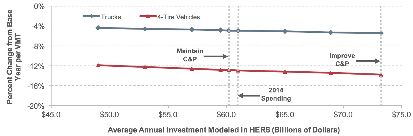
Exhibit 10-7 presents projections for vehicle operating costs per VMT, including separate values for four-tire vehicles (light-duty vehicles) and trucks (heavy-duty vehicles). The projected impacts on vehicle operating costs are larger for four-tire vehicles than for trucks when compared with both the 2014 values and the adjusted baseline. When comparing the vehicle operating cost projections with the adjusted baseline, the magnitudes of the impacts are much larger; isolating the effects of future highway investment reveals that vehicle operating costs per mile are projected to decline by between 11.8 percent and 13.7 percent for four-tire vehicles, and by between 4.3 percent and 5.4 percent for trucks from 2014 to 2034.
Exhibit 10-7: Projected Impact of Alternative Investment Levels on 2034 Vehicle Operating Costs on Federal-aid Highways
| HERS-Modeled Investment on Federal-aid Highways Average Annual Investment (Billions of 2014 Dollars) | Projected 2032 Performance Measures on Federal-Aid Highways | Link to Chapter 7 Scenario | |||||
|---|---|---|---|---|---|---|---|
| Average Vehicle Operating Costs | Percent Change Relative to Baseline | ||||||
| All Vehicles ($/VMT) | 4-Tire Vehicles ($/VMT) | Trucks ($/VMT) | 4-Tire Vehicles | Trucks | |||
| $73.2 | $0.418 | $0.342 | $1.034 | -13.7% | -5.4% | Improve C&P | |
| $68.9 | $0.419 | $0.343 | $1.035 | -13.4% | -5.2% | ||
| $65.0 | $0.420 | $0.344 | $1.037 | -13.2% | -5.1% | ||
| $61.0 | $0.421 | $0.346 | $1.039 | -12.9% | -4.9% | ||
| $60.2 | $0.422 | $0.346 | $1.039 | -12.8% | -4.9% | 2014 Spending | |
| $59.5 | $0.422 | $0.346 | $1.040 | -12.8% | -4.8% | Maintain C&P | |
| $57.0 | $0.423 | $0.347 | $1.041 | -12.5% | -4.7% | ||
| $53.0 | $0.424 | $0.348 | $1.043 | -12.2% | -4.5% | ||
| $49.0 | $0.426 | $0.350 | $1.046 | -11.8% | -4.3% | ||
| Base Year Values: | $0.466 | ||||||
Source: Highway Economic Requirements System.
The projected reductions in vehicle operating costs per VMT are driven by projected increases in fuel efficiency across the analysis horizon. The assumed paths of fuel efficiency are based on projections from the Energy Information Administration’s Annual Energy Outlook 2016. The average price of gasoline is assumed to increase between 2014 and 2034 by 0.7 percent relative to 2014, while the average price of diesel fuel is assumed to increase by 4.8 percent relative to 2014. The projected changes in fuel prices are added to the fuel cost savings that would result from the improvements in vehicle energy efficiency that the Energy Information Administration projects for this same period; these changes are represented in HERS as increases in average miles per gallon of 55.4 percent for light-duty vehicles, 47.0 percent for six-tire trucks, and 13.9 percent for other trucks.
Impact of Future Investment on Future VMT
As discussed above, the travel demand elasticity features in HERS modify future VMT growth for each HPMS sample section based on changes to highway user costs. In the absence of information to the contrary, most previous C&P Reports assumed that the HPMS forecasts represented the level of travel that would occur if user costs did not change. This assumption was changed beginning with the 2015 C&P Report because the baseline VMT forecasts used in this report are now tied to a specific VMT forecasting model with known inputs. HERS is now programmed to assume that the baseline projections of future VMT already account for anticipated independent changes in user cost component values.
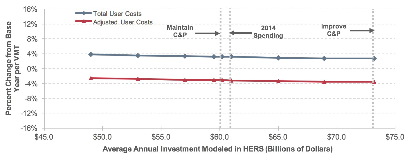
In computing the impact of user cost changes on future VMT growth on an HPMS sample section, HERS compares projected highway user costs against assumed user costs that would have occurred had the physical conditions or operating performance on that highway section remained unchanged. This concept is illustrated in Exhibit 10-8. Based on the 2014 values assigned to various user cost components (e.g., value of travel time per hour, fuel prices, fuel efficiency, truck travel as a percentage of total travel), HERS computes baseline 2014 user costs at $1.262 per mile. If the 2034 values assigned to those same user cost components were applied in 2014, however, HERS would compute 2014 user costs to be $1.344 per mile. This “adjusted baseline” is the relevant point of comparison when examining the impact of user cost changes on VMT.
Although user costs are projected to increase in absolute terms from 2014 to 2034, they are projected to decline relative to the adjusted baseline by between 2.6 percent (at the lowest level of investment analyzed) and 3.6 percent (at the highest level of investment analyzed in 2034). Because the percentage change in adjusted total user costs declined for each investment level identified, the effective annual projected VMT growth associated with each investment level was higher than the 1.07 percent baseline projection in all cases, ranging from 1.13 percent to 1.22 percent.
Impacts of NHS Investments Modeled by HERS
As described in Chapter 1, the NHS includes the Interstate System and other routes most critical to national defense, mobility, and commerce. As noted earlier, the NHS analyses presented in this section are based on the NHS after its expansion pursuant to MAP-21.
This section examines the impacts that investment on NHS roads could have on future NHS conditions and performance, independent of spending on other Federal-aid highways. The analysis presented in this section centers on special HERS runs that used a database consisting only of NHS roads. The highest two investment levels shown in the three exhibits presented in this section are based on model runs constrained by a BCR. The top row in each table represents a run within which all potential improvements with a BCR of 1.0 or higher are implemented; this corresponds to the definition of the Improve Conditions and Performance scenario presented in Chapter 7. The second row in each table represents a run at which the average annual investment level over 20 years matches actual 2014 highway capital spending by all levels of government combined. (HERS was unable to identify $44.0 billion of cost-beneficial investment annually assuming spending remained at this fixed amount in each year, so the analysis was redone as a BCR-constrained run under which spending varies by year.) The remaining investment levels presented in this section reflect analyses in which a fixed amount of investment occurred in each year; these were arbitrarily selected as increments of $4.0 billion per year simply to show a wide range of alternatives.
Exhibit 10-8: Projected Impact of Alternative Investment Levels on 2034 User Costs and VMT on Federal-aid Highways
| HERS-Modeled Investment on Federal-aid Highways Average Annual Investment (Billions of 2014 Dollars) | Projected 2034 Indicators on Federal-aid Highways | Link to Chapter 7 Scenario | |||||
|---|---|---|---|---|---|---|---|
| Average Total User Costs1 | Projected VMT2 | ||||||
| ($/VMT) | Percent Change | Trillions of VMT | Annual Percent Change vs. 2014 | ||||
| vs. Actual 2014 | vs. Adjusted Baseline | ||||||
| $73.2 | $1.296 | 2.7% | -3.6% | 3.227 | 1.22% | Improve C&P | |
| $68.9 | $1.297 | 2.8% | -3.5% | 3.212 | 1.19% | ||
| $65.0 | $1.299 | 2.9% | -3.4% | 3.205 | 1.18% | ||
| $61.0 | $1.301 | 3.1% | -3.2% | 3.197 | 1.17% | ||
| $60.2 | $1.302 | 3.2% | -3.1% | 3.195 | 1.17% | 2014 Spending | |
| $59.5 | $1.302 | 3.2% | -3.1% | 3.194 | 1.16% | Maintain C&P | |
| $57.0 | $1.303 | 3.3% | -3.0% | 3.189 | 1.16% | ||
| $53.0 | $1.306 | 3.5% | -2.8% | 3.181 | 1.14% | ||
| $49.0 | $1.309 | 3.7% | -2.6% | 3.172 | 1.13% | ||
| Base Year Values: | $1.262 | 2.534 | 1.07% | ||||
| Adjusted Baseline: | $1.344 | ||||||
1 The computation of user costs includes several components (value of travel time per hour, fuel prices, fuel efficiency, truck travel as a percentage of total travel, etc.) that are assumed to change over time independently of future highway investment. The adjusted baseline applies the parameter values for 2034 to the data for 2014 so that changes in user costs attributable to future highway investment can be identified.
2 The operation of the travel demand elasticity features in HERS cause future VMT growth to be influenced by future changes in average user costs per VMT. For this report, the model was set to assume that the baseline projections of future VMT already take into account anticipated independent future changes in user cost component values; hence, it is the changes versus the adjusted baseline user costs that are relevant. Since the percentage change in adjusted total user costs declined for each of the investment levels identified, the annual projected VMT growth was higher than the 0.92-percent baseline projection in all cases.
Source: Highway Economic Requirements System.
Impact of Future Investment on NHS User Costs and VMT
Exhibit 10-9 presents the projected impacts of NHS investment on VMT and total average user costs on NHS roads in 2034. Average user costs are projected to be lower in 2034 than for the adjusted baseline ($1.262 per VMT) for all investment levels presented. When implementing all cost-beneficial projects (the highest level of investment, an annual average of $48.1 billion), average total user costs are projected to be 3.48 percent lower ($1.218 per VMT) than adjusted baseline user costs in 2014 ($1.262 per VMT). At the lowest level of investment presented (an annual average of $28.0 billion), average total user costs are projected to be 1.97 percent lower ($1.237 per VMT) than adjusted baseline user costs in 2014.
Projected VMT growth on NHS roads is relatively insensitive to the range of investment levels presented in Exhibit 10-9. At the highest level of investment presented in Exhibit 10-9 (an annual average of $48.1 billion), VMT is projected to grow at an average annual rate of 1.20 percent from 2014 to 2034 (2.086 trillion VMT in 2034 versus 1.644 trillion VMT in 2014). At the lowest level of investment presented in Exhibit 10-9 (an annual average of $28.0 billion), VMT is projected to grow at an average annual rate of 1.10 percent from 2014 to 2034 (2.046 trillion VMT in 2034 versus 1.644 trillion VMT in 2014).
Across the investment levels presented in Exhibit 10-9, HERS allocates between $18.0 billion and 29.6 billion in average annual spending on NHS roads to system rehabilitation and between $10.0 billion and $18.5 billion in average annual spending on NHS roads to system expansion.
Exhibit 10-9: HERS Investment Levels Analyzed for the National Highway System and Projected Minimum Benefit-Cost Ratios, User Costs, and Vehicle Miles Traveled
| HERS-Modeled Investment On the NHS (Average Annual Over 20 Years) | Projected NHS Indicators | Description | ||||
|---|---|---|---|---|---|---|
| Total HERS Spending1 | System Rehabilitation Spending | System Expansion Spending | Minimum BCR 20-Year 2015 through 20342 | Average 2034 Total User Costs ($/VMT)3 | Projected 2034 VMT (Trillions)4 | |
| $48.1 | $29.6 | $18.5 | 1.00 | $1.218 | 2.086 | BCR>=1.0 |
| $44.0 | $27.4 | $16.6 | 1.07 | $1.221 | 2.079 | 2014 Spending |
| $40.0 | $25.1 | $14.9 | 1.08 | $1.224 | 2.072 | |
| $36.0 | $22.9 | $13.1 | 1.16 | $1.228 | 2.064 | |
| $32.0 | $20.5 | $11.5 | 1.28 | $1.232 | 2.056 | |
| $28.0 | $18.0 | $10.0 | 1.42 | $1.237 | 2.046 | |
| Base Year Values: | $1.195 | 1.644 | ||||
| Adjusted Baseline: | $1.262 | |||||
1 HERS splits its available budget between system rehabilitation and system expansion based on the mix of spending it finds to be most cost-beneficial, which varies by funding level.
2 As HERS ranks potential improvements by their estimated BCRs and assumes that the improvements with the highest BCRs will be implemented first (up until the point where the available budget specified is exhausted), the minimum BCR will naturally tend to decline as the level of investment analyzed rises.
3 The computation of user costs includes several components (value of travel time per hour, fuel prices, fuel efficiency, truck travel as a percentage of total travel, etc.) that are assumed to change over time independently of future highway investment. The adjusted baseline applies the parameter values for 2034 to the data for 2014, so that changes in user costs attributable to future highway investment can be identified.
4 The operation of the travel demand elasticity features in HERS cause future VMT growth to be influenced by future changes in average user costs per VMT. For this report, the model was set to assume that the baseline projections of future VMT already take into account anticipated independent future changes in user cost component values; hence, it is the changes versus the adjusted baseline user costs that are relevant.
Source: Highway Economic Requirements System.
Impact of Future Investment on NHS Travel Times and Travel Time Costs
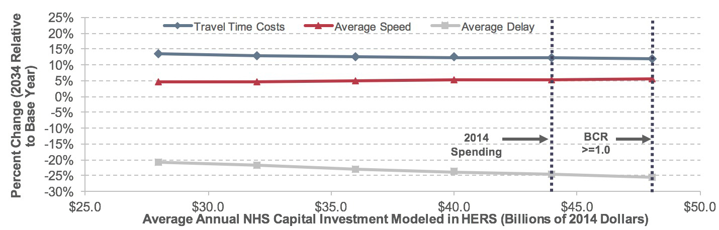
The tabular portion of Exhibit 10-10 presents the projections of NHS averages for time-related indicators of performance, along with the spending amount that HERS allocates for NHS expansion projects (which have stronger effects on time-related indicators of performance than preservation projects have).
The graph is plotted based on total average annual NHS investment modeled in HERS, including spending on both system rehabilitation and system expansion. For all investment levels presented in Exhibit 10-10, average travel speed in 2034 exceeds average travel speed in 2014 (49.6 miles per hour). The range of average travel speeds is narrow across the investment levels. At the lowest level of investment in system expansion presented in Exhibit 10-10 (an annual average of $11.5 billion), the average travel speed in 2034 is projected to be 52.0 miles per hour. At the highest level of investment in system expansion presented in Exhibit 10-10 (an annual average of $18.5 billion), the average travel speed in 2034 is projected to be 52.4 miles per hour.
The global increase in average travel speed across investment levels corresponds to large decreases in average delay per VMT across investment levels. At the highest level of investment in system expansion presented in Exhibit 10-10, average delay per VMT in 2034 is projected to be 25.4 percent lower than in 2014. At the lowest level of investment in system expansion presented in Exhibit 10-10, average delay per VMT in 2034 is projected to be 21.8 percent lower than in 2014.
Exhibit 10-10: Projected Impact of Alternative Investment Levels on 2034 Highway Speed, Travel Delay, and Travel Time Costs on the National Highway System
| HERS-Modeled Investment on the NHS Average Annual Spending (Billions of 2014 Dollars) |
Projected 2034 Performance Measures on the NHS | Description | ||||
|---|---|---|---|---|---|---|
| Average Speed (mph) | Percent Change Relative to Baseline | |||||
| Total | System Expansion1 |
Average Speed | Average Delay per VMT | Travel Time Costs per VMT2 | ||
| $48.1 | $18.5 | 52.4 | 5.5% | -25.4% | 11.9% | BCR>=1.0 |
| $44.0 | $16.6 | 52.3 | 5.3% | -24.5% | 12.1% | 2014 Spending |
| $40.0 | $14.9 | 52.2 | 5.2% | -23.8% | 12.4% | |
| $36.0 | $13.1 | 52.1 | 5.0% | -22.9% | 12.7% | |
| $32.0 | $11.5 | 52.0 | 4.7% | -21.8% | 13.0% | |
| $27.0 | $9.6 | 51.8 | 4.4% | -20.4% | 13.5% | |
| Base Year Values: | 49.6 | |||||
1 The amounts shown represent only the portion of HERS-modeled spending directed toward system expansion, rather than system rehabilitation. Other types of spending can affect these indicators as well.
2 Travel time costs are affected by an assumption that the value of time will increase by 1.0 percent in real terms each year. Hence, costs would rise even if travel time remained constant.
Source: Highway Economic Requirements System; Highway Statistics 2015, Table VM-1.
Travel time costs per VMT in 2034 are projected to increase across the investment levels presented. Travel time costs per VMT in 2034 are projected to increase by 11.9 percent relative to 2014 at the highest investment level and to increase by 13.0 percent at the lowest level of investment.
Impact of Future Investment on NHS Pavement Ride Quality
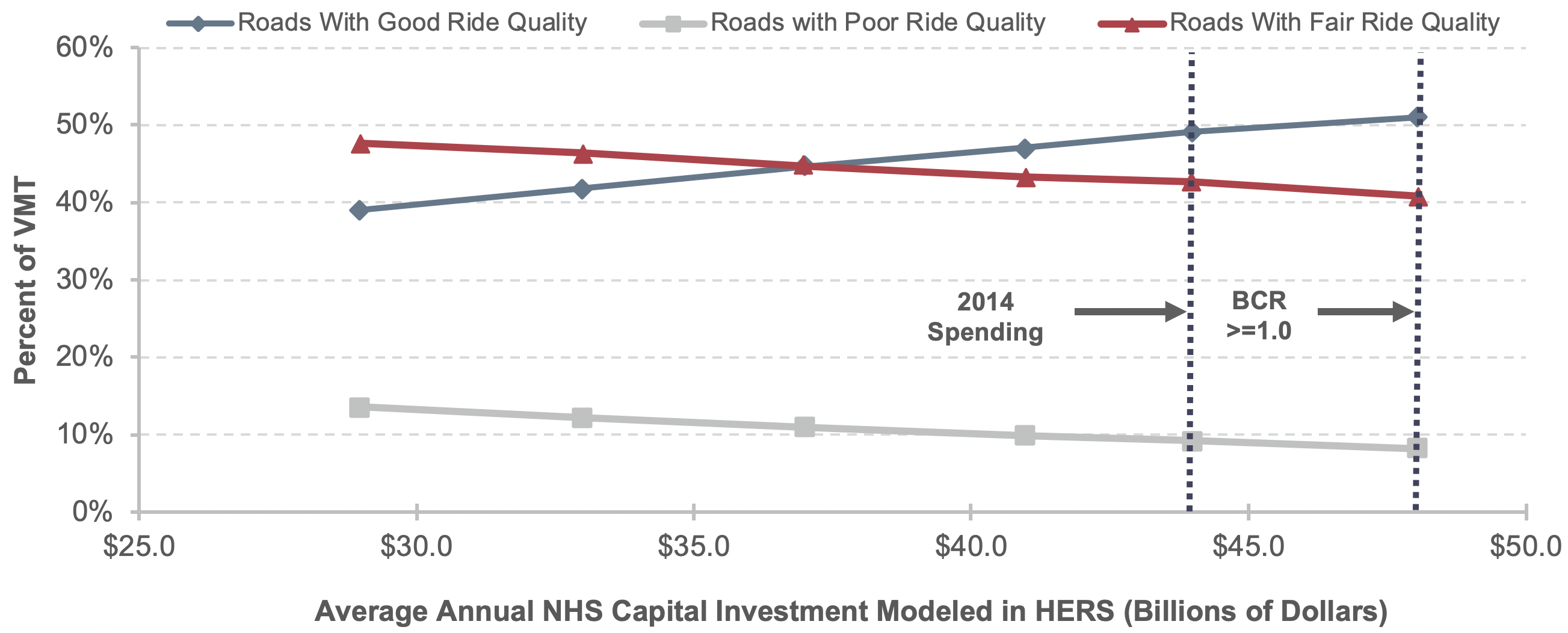
The tabular portion of Exhibit 10-11 shows the portion of modeled NHS spending that HERS allocates to rehabilitation projects (which influence average pavement quality more than expansion projects do). The graph is plotted based on total average annual NHS investment modeled in HERS, including spending on both system rehabilitation and system expansion. At the highest level of investment presented in Exhibit 10-11 (an annual average of 29.6 billion allocated to system rehabilitation), the model projects that pavements with an IRI above 170 (the criterion presented in Chapter 6 for rating ride quality as “poor”) will carry 8.2 percent of the VMT on the NHS, down from the 11.4 percent estimated for 2014.
HERS also projects the share of travel on pavements with an IRI below 95 (the criterion presented in Chapter 6 for rating ride quality as “good”) will carry 51.0 percent of the VMT on the NHS, down from the 58.7 percent estimated for 2014. The model projects a large increase in the share of NHS travel on pavements with “fair” ride quality (rising from 30.0 percent in 2014 to projects in 2034), and projects the average IRI of the system would rise 3.6 percent to 105.6, remaining within the classification of providing “fair” ride quality at the aggregate level.
Based on these modeling results, additional investment to bring the percentage of NHS VMT on roads with “good” ride quality closer to 100 percent would be economically inefficient, as the costs would exceed the benefits. As discussed in Chapter 6, while the percentage of VMT on pavements with good ride quality has improved significantly over the past decade, other measures of pavement performance have shown declines. The HERS results suggest that some degree of shifting of pavement investment (toward lower-volume NHS routes, or non-NHS routes) may be warranted.
The model does find it to be cost-beneficial to reduce the share of pavements with poor ride quality, but not all the way down to zero percent. A key factor leading to this result is that some improvements are not cost-beneficial until IRI rises above the threshold for “fair” ride quality by a sufficient margin. Thus, for some roads with an IRI above 170, improvements would not generate benefits exceeding costs. Also, at any given point, some pavements will be under construction, which will negatively affect their ride quality.
At the lowest level of investment presented in Exhibit 10-11 (an annual average of $18.7 billion allocated to system rehabilitation), the model projects that the share of NHS travel carried by pavements with an IRI above 170 would rise from 11.4 percent in 2014 to 13.6 percent in 2034. At this investment level, average IRI would increase to 121.3, and the share of NHS travel on pavements with an IRI below 95 would decline to 39.1 percent.
Exhibit 10-11: Projected Impact of Alternative Investment Levels on 2034 Pavement Ride Quality Indicators for the National Highway System
| HERS-Modeled Investment on the NHS Average Annual Spending (Billions of 2014 Dollars) | Projected 2034 Condition Measures on the NHS1 | Description | |||||
|---|---|---|---|---|---|---|---|
| Percent of VMT on Roads With Ride Quality of: | Average IRI (VMT-Weighted) | ||||||
| Total | System Rehabilitation2 | Good (IRI<95) | Fair (IRI 95 to 170) |
Poor (IRI>170) |
Inches Per Mile | Change Relative to Base Year | |
| $48.1 | 29.6 | 51.0% | 40.7% | 8.2% | 105.6 | 3.6% | BCR>=1.0 |
| $44.0 | $27.4 | 49.1% | 41.7% | 9.2% | 107.9 | 5.9% | 2014 Spending |
| $41.0 | $25.7 | 47.0% | 43.0% | 9.9% | 110.9 | 8.8% | |
| $37.0 | $23.5 | 44.6% | 44.4% | 11.0% | 113.8 | 11.7% | |
| $33.0 | $21.2 | 41.8% | 46.0% | 12.1% | 117.3 | 15.1% | |
| $29.0 | $18.7 | 39.1% | 47.3% | 13.6% | 121.3 | 19.0% | |
| Base Year Values: | 58.7% | 30.0% | 11.4% | 101.9 | |||
1 As discussed in Chapter 6, IRI values of 95 through 170 inches per mile are classified as “fair,” lower IRI values are classified as “good,” and higher IRI values are classified as “poor.”
2 The amounts shown represent only the portion of HERS-modeled spending directed toward system rehabilitation, rather than system expansion. Other types of spending can affect these indicators as well.
Source: Highway Economic Requirements System.
Impacts of Interstate System Investments Modeled by HERS
The Interstate System, unlike the broader NHS of which it is a part, has standard design and signage requirements, making it the most recognizable subset of the highway network. This section examines the impacts that investment in the Interstate System could have on future Interstate System conditions and performance, independently of spending on other Federal-aid highways. The analysis presented in this section centers on special HERS runs that used a database consisting only of Interstate System roads.
As was the case for the NHS analyses presented above, the highest two investment levels shown in the three exhibits presented in this section are based on model runs constrained by a BCR. The top row in each table represents a run with in which all potential improvements with a BCR of 1.0 or higher are implemented; this corresponds to the definition of the Improve Conditions and Performance scenario presented in Chapter 7. The second row in each table represents a run at which the average annual investment level over 20 years matches actual 2014 highway capital spending by all levels of government combined. (HERS was unable to identify $20.3 billion of cost-beneficial investment annually assuming spending remained at this fixed amount in each year, so the analysis was redone as a BCR-constrained run under which spending varies by year.) The remaining investment levels presented in this section reflect analyses in which a fixed amount of investment occurred in each year; these were arbitrarily selected simply to show a wide range of alternatives.
Impact of Future Investment on Interstate User Costs and VMT
Exhibit 10-12 presents the projected impacts of highway investment on VMT and total average user costs on Interstate roads in 2034, along with the amount that HERS allocates to Interstate projects. Average user costs are projected to be lower in 2034 than the adjusted baseline ($1.162 per VMT) for all investment levels presented. At the highest level of investment presented in Exhibit 10-12 (an annual average of $21.3 billion), average total user costs are projected to be 2.5 percent lower ($1.133 per VMT) than in 2014. At the lowest level of investment presented (an annual average of $11.5 billion), average total user costs are projected to be 0.03 percent lower ($1.159 per VMT) than in 2014.
Exhibit 10-12: HERS Investment Levels Analyzed for the Interstate System and Projected Minimum Benefit-Cost Ratios, User Costs, and Vehicle Miles Traveled
| HERS-Modeled Investment On the Interstate System | Projected Interstate Indicators | Description | ||||
|---|---|---|---|---|---|---|
| Average Annual Over 20 Years | Minimum BCR 20-Year 2015 through 20342 | Average 2034 Total User Costs ($/VMT)3 | Projected 2034 VMT (Trillions)4 | |||
| Total HERS Spending1 | System Rehabilitation Spending | System Expansion Spending | ||||
| $21.3 | $11.9 | $9.3 | 1.00 | $1.133 | 0.940 | BCR>=1.0 |
| $20.3 | $11.7 | $8.6 | 1.06 | $1.136 | 0.938 | 2014 Spending |
| $15.5 | $9.4 | $6.1 | 1.10 | $1.149 | 0.930 | |
| $14.5 | $8.8 | $5.7 | 1.15 | $1.151 | 0.928 | |
| $13.5 | $8.3 | $5.2 | 1.23 | $1.154 | 0.926 | |
| $12.5 | $7.7 | $4.8 | 1.32 | $1.157 | 0.924 | |
| $11.5 | $7.1 | $4.4 | 1.43 | $1.159 | 0.921 | |
| Base Year Values: | $1.115 | 0.738 | ||||
| Adjusted Baseline: | $1.162 | |||||
1 HERS splits its available budget between system rehabilitation and system expansion based on the mix of spending it finds to be most cost-beneficial, which varies by funding level.
2 As HERS ranks potential improvements by their estimated BCRs, and assumes that the improvements with the highest BCRs will be implemented first (up until the point where the available budget specified is exhausted), the minimum BCR will naturally tend to decline as the level of investment analyzed rises.
3 The computation of user costs includes several components (value of travel time per hour, fuel prices, fuel efficiency, truck travel as a percent of total travel, etc.) that are assumed to change over time independent of future highway investment. The adjusted baseline applies the parameter values for 2034 to the data for 2014 so that changes in user costs attributable to future highway investment can be identified.
4 The operation of the travel demand elasticity features in HERS cause future VMT growth to be influenced by future changes in average user costs per VMT. For this report, the model was set to assume that the baseline projections of future VMT already take into account anticipated independent future changes in user cost component values; hence, it is the changes versus the adjusted baseline user costs that are relevant.
Source: Highway Economic Requirements System.
Projected VMT growth on Interstate highways is relatively insensitive to the range of investment levels presented in Exhibit 10-12. At the highest level of investment presented in Exhibit 10-12 (an annual average of $23.7 billion), VMT is projected to grow at an average annual rate of 1.22 percent from 2014 to 2034 (940 billion VMT in 2034 versus 738 billion VMT in 2014). At the lowest level of investment presented in Exhibit 10-12 (an annual average of $11.2 billion), VMT is projected to grow at an average annual rate of 1.11 percent from 2014 to 2034 (921 billion VMT in 2034 versus 738 billion VMT in 2014).
Across the investment levels presented in Exhibit 10-12, HERS allocates between $7.1 billion and $11.9 billion in average annual spending on Interstate roads to system rehabilitation, and between $4.4 billion and $9.3 billion in average annual spending on Interstate roads to system expansion.
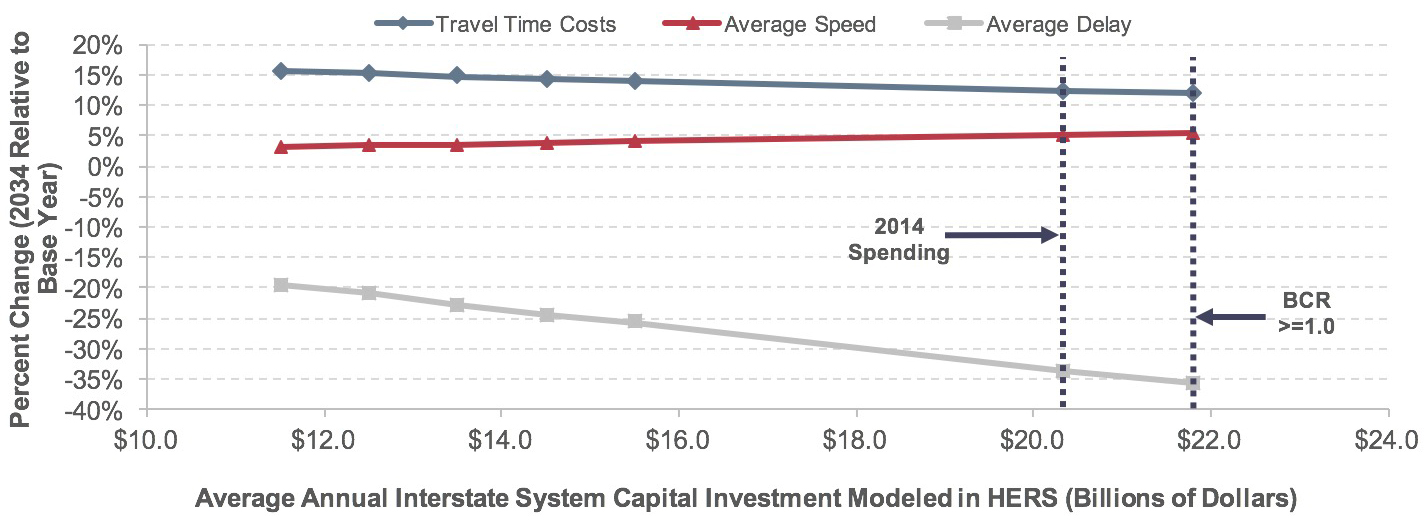
Impact of Future Investment on Interstate System Travel Times and Travel Costs
The tabular portion of Exhibit 10-13 presents the projections of Interstate System averages for time-related indicators of performance, along with the amount that HERS allocates for Interstate System expansion projects (which have a relatively large impact on travel time). The graph is plotted based on total average annual Interstate investment modeled in HERS, including spending on both system rehabilitation and system expansion.
Exhibit 10-13: Projected Impact of Alternative Investment Levels on 2034 Highway Speed, Travel Delay, and Travel Time Costs on the Interstate System
| HERS-Modeled Investment on Interstate Highways | Projected 2034 Performance Measures on Interstate Highways | Description | ||||
|---|---|---|---|---|---|---|
| Average Annual Spending (Billions of 2014 Dollars) | Average Speed (mph) | Percent Change Relative to Baseline | ||||
| Average Speed | Average Delay per VMT | Travel Time Costs per VMT2 | ||||
| Total | System Expansion1 | |||||
| $21.3 | $9.3 | 65.6 | 5.5% | -35.7% | 12.2% | BCR>=1.0 |
| $20.3 | $8.6 | 65.4 | 5.2% | -33.8% | 12.5% | 2014 Spending |
| $15.5 | $6.1 | 64.7 | 4.1% | -25.6% | 14.1% | |
| $14.5 | $5.7 | 64.6 | 4.0% | -24.4% | 14.4% | |
| $13.5 | $5.2 | 64.4 | 3.6% | -22.8% | 14.8% | |
| $12.5 | $4.8 | 64.2 | 3.3% | -20.7% | 15.3% | |
| $11.5 | $4.4 | 64.1 | 3.1% | -19.6% | 15.6% | |
| Base Year Values: | 62.2 | |||||
1 The amounts shown represent only the portion of HERS-modeled spending directed toward system expansion, rather than system rehabilitation. Other types of spending can affect these indicators as well.
2 Travel time costs are affected by an assumption that the value of time will increase by 1.0 percent in real terms each year; hence, costs would rise even if travel time remained constant.
Source: Highway Economic Requirements System; Highway Statistics 2015, Table VM-1.
Across all investment levels presented in Exhibit 10-13, average speed on the Interstate System is projected to be higher than its 2014 level (62.2 miles per hour) in 2034. At the highest level of investment presented in Exhibit 10-13 (average annual investment in system expansion of $9.3 billion), average Interstate highway travel speed is projected to be 5.5 percent higher (65.6 miles per hour) in 2034 than in 2014. At the lowest level of investment presented in Exhibit 10-13 (average annual investment in system expansion of $4.4 billion), average Interstate highway travel speed is projected to be 3.1 percent higher (64.1 miles per hour) in 2034 than in 2014.
The global increase in average travel speed across investment levels corresponds with large decreases in average delay per VMT across investment levels. At the highest level of investment presented in Exhibit 10-13, average delay per VMT in 2034 is projected to be 35.7 percent lower than in 2014. At the lowest level of investment presented in Exhibit 10-13, average delay per VMT in 2034 is projected to be 19.6 percent lower than in 2014.
The projected impacts on travel delay across investment levels are much greater for Interstates than for other portions of Federal-aid highways. This result suggests the presence of a large scope of congestion-related benefits that could be achieved through investments in Interstate highway improvements.
Due to increases in the assumed value of time from 2014 to 2034 as discussed earlier under Impact of Future Investment on Highway Pavement Ride Quality, the projected increases in average travel speed do not correspond to decreases in travel time costs per VMT. Travel time costs per VMT in 2034 are projected to increase across all investment levels. Travel time costs per VMT in 2034 are projected to increase by 12.2 percent relative to 2014 at the highest level of investment presented in Exhibit 10-13 and by 15.6 percent at the lowest level of investment.
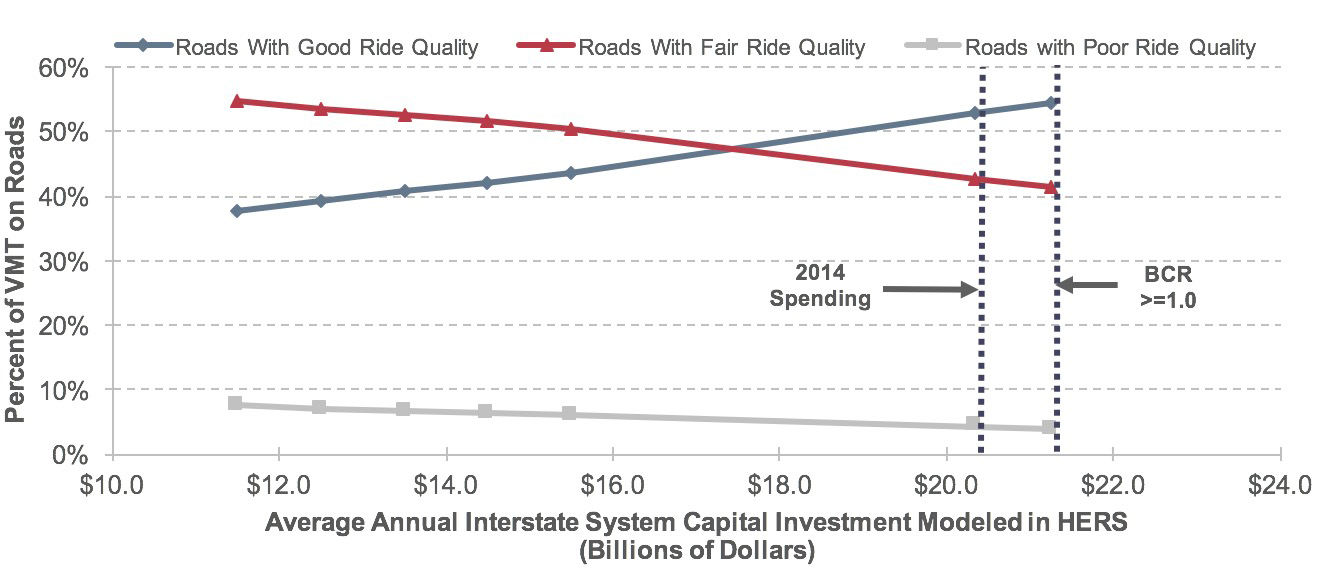
Impact of Future Investment on Interstate Pavement Ride Quality
The tabular portion of Exhibit 10-14 shows the portions of modeled Interstate System spending that HERS allocates to rehabilitation projects (which influence average pavement quality more than expansion projects do). The graph is plotted based on total average annual Interstate investment modeled in HERS, including spending on both system rehabilitation and system expansion. Across all investment levels presented in Exhibit 10-14, the model projects that the share of pavements with an IRI below 95 (the criterion described in Chapter 6 for rating ride quality as “good”) would be below the corresponding share in 2014 (72.2 percent). These results suggest that placing more emphasis on reducing the percentage of VMT on Interstate highways with “poor” ride quality would be more economically efficient than focusing on further increasing the share with “good” ride quality. A key factor leading to this result is that HERS assumes that the effects of increasing pavement roughness on free-flow speed and vehicle operating costs are modest until after IRI rises to a relatively high level.
At the highest level of investment presented in Exhibit 10-14 (an annual average of $11.9 billion allocated to system rehabilitation), the model projects average pavement roughness on the Interstate System to be 11.5 percent higher in 2034 than in 2014. These results suggest that it would not be cost-effective to keep the average VMT-weighted IRI of the Interstate System at its 2014 level of 85.9 (well into the “good” range), and that allowing it to move just across the threshold into the “fair” range (to 95.8) would be economically advantageous. The HERS results also suggest it would not be cost-beneficial to reduce the percent of Interstate VMT on pavements with “good” ride quality below its 2014 level of 4.0 percent.
Exhibit 10-14: Projected Impact of Alternative Investment Levels on 2034 Pavement Ride Quality Indicators for the Interstate System
| HERS-Modeled Investment on Interstate Highways | Projected 2034 Condition Measures Interstate Highways1 | Description | |||||
|---|---|---|---|---|---|---|---|
| Average Annual Spending (Billions of 2014 Dollars) |
Percent of VMT on Roads with Ride Quality of: | Average IRI (VMT-Weighted) | |||||
| Total | System Rehabilitation2 |
Good (IRI<95) | Fair (IRI 95 to 170) | Poor (IRI>170) | Inch Per Mile | Chan to Base Year | |
| $21.3 | $11.9 | 54.4% | 41.5% | 4.0% | 95.8 | 11.5% | BCR>=1.0 |
| $20.3 | $11.7 | 52.8% | 42.8% | 4.4% | 97.2 | 13.2% | 2014 Spending |
| $15.5 | $9.4 | 43.7% | 50.3% | 6.0% | 105.6 | 22.9% | |
| $14.5 | $8.8 | 42.0% | 51.6% | 6.4% | 107.1 | 24.7% | |
| $13.5 | $8.3 | 40.7% | 52.6% | 6.7% | 108.4 | 26.2% | |
| $12.5 | $7.7 | 39.3% | 53.5% | 7.1% | 109.7 | 27.7% | |
| $11.5 | $7.1 | 37.7% | 54.6% | 7.7% | 111.6 | 29.9% | |
| Base Year Values: | 72.2% | 23.8% | 4.0% | 85.9 | |||
1 As discussed in Chapter 6, IRI values of 95 through 170 inches per mile are classified as “fair,” lower IRI values are classified as “good,” and higher IRI values are classified as “poor.”
2 The amounts shown represent only the portion of HERS-modeled spending directed toward system rehabilitation, rather than system expansion. Other types of spending can affect these indicators as well.
Source: Highway Economic Requirements System.
Impacts of Systemwide Investments Modeled by NBIAS
In using NBIAS to project conditions and performance of the Nation’s bridges over 20 years, this section considers the alternatives of continuing to invest in bridge rehabilitation at the 2014 level (in constant dollars) and at higher or lower levels. The expenditures modeled pertain only to bridge system rehabilitation; expenditures associated with bridge system expansion are modeled separately as part of the capacity expansion analysis in HERS. The NBIAS-modeled investments presented here should be considered as additive to the HERS-modeled investments presented above; each capital investment scenario presented in Chapter 7 combines one HERS analysis with one NBIAS analysis and makes adjustments to account for nonmodeled spending.
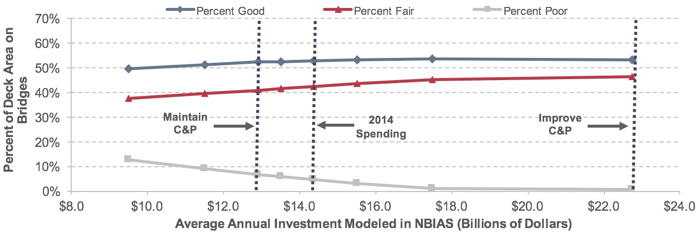
As referenced in Chapter 2, of the $105.4 billion invested in highways in 2014, $14.4 billion was used for bridge system rehabilitation. For investments of the types modeled by NBIAS, Exhibit 10-15 shows how the total amount invested over the 20-year analysis period influences the bridge performance levels projected for the final year, 2034. If spending were sustained at its 2014 level in constant dollar terms ($14.4 billion, the investment level feeding the 2014 Spending scenario presented in Chapter 7), projected performance for 2034 would improve relative to 2014 for each performance measure considered. The share of bridges classified as in “poor” condition would decrease from 6.8 percent to 4.7 percent, while the share of bridges classified as in “good” condition would increase from 44.3 percent in 2014 to 52.8 percent in 2034. The average Health Index would rise from 92.1 to 94.3. The Economic Investment Backlog would decrease to $49.5 billion (60.5 percent below its 2014 level of $125.4 billion).
The highest level of spending shown in Exhibit 10-15 averages $22.7 billion per year (this feeds the Improve Conditions and Performance scenario in Chapter 7). This level of investment is projected to reduce the deck-area-weighted share of bridges in poor condition to 0.6 percent and to eliminate the Economic Investment Backlog for bridges by 2034. This indicates that the model does not find that completely eliminating all deficiencies would be cost-beneficial at any single point in time. In some cases, the model recommends that corrective actions be deferred; in other cases it estimates that the benefits of replacing a bridge would be outweighed by its costs (suggesting that it should eventually be closed, diverting traffic to other available crossings).
Bridge Performance Measures in Exhibits 10-15 to 10-18
Exhibits 10-15 to 10-18 provide three metrics of bridge performance:
- Percentage of bridges (weighted by deck area) in “good,” “fair,” and “poor” condition (the percentage in poor condition is used in computing the Maintain Conditions and Performance scenario in Chapter 7)
- Average Health Index
- Economic Investment Backlog (used in computing the Improve Conditions and Performance scenario in Chapter 7)
As described in Chapter 6, bridges in “good,” “fair,” and “poor” condition are defined by the degree of deterioration of the three major bridge components: deck, superstructure, and substructure. For a bridge to be classified as in “good” condition, all three major bridge components must be rated “good.” For a bridge to be classified as in “poor” condition, at least one bridge element must be rated “poor.” All other bridges are classified as in “fair” condition.
The average Health Index metric is a ranking system (0–100) for bridge elements typically used in the context of decisionmaking for bridge preventive maintenance, with 0 being the worst and 100 being the best. To aggregate the element-level result to the bridge level (i.e., assign a value for the Health Index), a weight is assigned to each bridge element according to the economic consequences of its failure, and then an average of all the weighted elements is calculated. Thus, an element for which a failure has relatively little economic effect would receive less weight than an element for which a failure could result in closing the bridge. In general, the lower the Health Index, the higher the priority for rehabilitation or maintenance of the structure, although other factors also are instrumental in determining priority of work on bridges.
The Economic Investment Backlog metric represents the combined cost of all corrective actions for which NBIAS estimates implementation would be cost-beneficial. Consistent with the HERS analysis, implementing all cost-beneficial corrective actions in NBIAS would not necessarily mean that no bridges would remain in poor condition; rather, implementing all cost-beneficial corrective actions in NBIAS would indicate that it would not be cost-beneficial to take any further corrective actions.
Exhibit 10-15: Projected Impact of Alternative Investment Levels on 2034 Bridge Condition Indicators for All Bridges
| NBIAS-Modeled Investment on All Bridges | Projected 2034 Condition Indicators—All Bridges | Link to Chapter 7 Scenario | ||||
|---|---|---|---|---|---|---|
| Average Annual Investment (Billions of 2014 Dollars)1 | Weighted by Deck Area | Health Index | Economic Investment Backlog (Billions of 2014 Dollars)1 | |||
| Percent Good | Percent Fair | Percent Poor | ||||
| $22.7 | 53.0% | 46.3% | 0.6% | 95.2 | $0.0 | Improve C&P |
| $17.5 | 53.8% | 45.0% | 1.2% | 95.2 | $4.3 | |
| $15.5 | 53.3% | 43.5% | 3.2% | 94.9 | $30.7 | |
| $14.4 | 52.8% | 42.5% | 4.7% | 94.3 | $49.5 | 2014 Spending |
| $13.5 | 52.5% | 41.5% | 5.9% | 93.7 | $64.7 | |
| $12.9 | 52.2% | 40.9% | 6.8% | 93.3 | $75.6 | Maintain C&P |
| $11.5 | 51.3% | 39.6% | 9.2% | 92.2 | $101.3 | |
| $9.5 | 49.4% | 37.7% | 12.9% | 90.3 | $141.6 | |
| Base Year Values: | 44.3% | 48.9% | 6.8% | 92.1 | $125.4 | |
1 The amounts shown do not reflect system expansion needs; the bridge components of such needs are addressed as part of the HERS model analysis.
Source: National Bridge Investment Analysis System.
Exhibit 10-15 also indicates that the average annual bridge investment could be reduced from the 2014 level while maintaining bridge performance. The Maintain C&P scenario (an average annual spending of $12.9 billion) would still be sufficient to maintain the share of bridges in poor condition, weighted by deck area, at 6.8 percent (its 2014 level) through 2034. At this level of investment, the average Health Index is projected to rise 1.2 percentage points (improve), and the Economic Investment Backlog is projected to shrink (improve) from $125.4 billion to $75.6 billion.
Impacts of Federal-aid Highway Investments Modeled by NBIAS
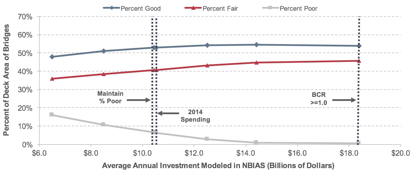
For bridges on Federal-aid highways, Exhibit 10-16 compares performance projections for 2034 at various levels of investment with measured performance in 2014. If spending on the types of improvements modeled in NBIAS were sustained at the 2014 level of $10.5 billion (in constant dollars), performance is projected to improve slightly. The percent of bridges in “poor” condition would decrease from 6.5 percent to 6.3 percent weighted by deck area, and the average Health Index would rise from 92.1 to 93.4. The Economic Investment Backlog would decrease by 59.3 percent (to $60.6 billion) from its 2014 level of $102.2 billion.
Exhibit 10-16: Projected Impact of Alternative Investment Levels on 2034 Bridge Condition Indicators for Federal-aid Highway Bridges
| NBIAS-Modeled Investment on Federal-aid Bridges | Projected 2034 Condition Indicators—Federal-aid Bridges | Link to Chapter 7 Scenario | ||||
|---|---|---|---|---|---|---|
| Average Annual Investment (Billions of 2014 Dollars)1 | Weighted by Deck Area | Health Index | Economic Investment Backlog (Billions of 2014 Dollars)1 | |||
| Percent Good | Percent Fair | Percent Poor | ||||
| $18.4 | 53.9% | 45.6% | 0.5% | 95.2 | $0.0 | BCR>=1.0 |
| $14.4 | 54.5% | 44.6% | 0.8% | 95.3 | $0.6 | |
| $12.5 | 54.0% | 43.0% | 2.9% | 94.9 | $25.0 | |
| $10.5 | 52.9% | 40.8% | 6.3% | 93.4 | $60.6 | 2014 Spending |
| $10.4 | 52.9% | 40.7% | 6.5% | 93.3 | $62.0 | Maintain % Poor |
| $8.5 | 51.0% | 38.3% | 10.6% | 91.3 | $100.3 | |
| $6.5 | 47.8% | 36.0% | 16.2% | 88.4 | $146.9 | |
| Base Year Values: | 43.3% | 50.2% | 6.5% | 92.1 | $102.2 | |
1 The amounts shown do not reflect system expansion needs; the bridge components of such needs are addressed as part of the HERS model analysis.
Source: National Bridge Investment Analysis System.
At the $18.4 billion average annual investment level feeding the Improve Conditions and Performance scenario, NBIAS projects the percent of bridges in “poor” condition weighted by deck area would decrease to 0.5 percent on Federal-aid highways. The Economic Investment Backlog would be reduced to zero by 2034, and the Average Health Index would increase from 92.1 to 95.2.
Impacts of NHS Investments Modeled by NBIAS
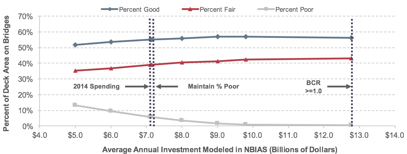
The impact of various funding levels on the performance of the bridges on the NHS is shown in Exhibit 10-17.
If spending on types of improvements modeled in NBIAS on NHS bridges were sustained at the 2014 level of $10.5 billion ($7.1 billion in constant dollar terms), the deck-area-weighted share of bridges in “poor” condition would increase slightly from 5.8 percent in 2014 to 5.8 percent in 2034. The average annual investment needed to maintain this indicator at its 2014 level is slightly higher (also rounding to $7.1 billion per year). This finding deviates from those identified above for all bridges and bridges on Federal-aid highways, for which spending in 2014 was estimated to be above the level needed to maintain this metric at base year levels. For the Improve C&P scenario, the average annual investment level of $7.1 billion would reduce the Economic Investment Backlog to zero by 2034. The percentage of bridges in “poor” condition would decrease from 5.8 in 2014 to 0.4 percent in 2034. The average Health Index would increase from 92.1 to 95.3 during the same period.
Exhibit 10-17: Projected Impact of Alternative Investment Levels on 2034 Bridge Condition Indicators for Bridges on the National Highway System
| NBIAS-Modeled Investment on NHS Bridges | Projected 2034 Condition Indicators—NHS Bridges | Link to Chapter 7 Scenario | ||||
|---|---|---|---|---|---|---|
| Average Annual Investment (Billions of 2014 Dollars)1 | Weighted by Deck Area | Health Index | Economic Investment Backlog (Billions of 2014 Dollars)1 | |||
| Percent Good | Percent Fair | Percent Poor | ||||
| $12.8 | 56.3% | 43.3% | 0.4% | 95.3 | $0.0 | BCR>=1.0 |
| $9.8 | 56.9% | 42.3% | 0.8% | 95.3 | $0.7 | |
| $9.0 | 56.8% | 41.4% | 1.8% | 95.3 | $8.3 | |
| $8.0 | 55.9% | 40.4% | 3.7% | 94.6 | $24.4 | |
| $7.1 | 55.2% | 39.0% | 5.8% | 93.6 | $40.3 | Maintain % Poor |
| $7.1 | 55.2% | 38.9% | 5.9% | 93.5 | $41.2 | 2014 Spending |
| $6.0 | 53.7% | 36.8% | 9.5% | 92.0 | $63.9 | |
| $5.0 | 51.6% | 35.2% | 13.2% | 90.0 | $87.2 | |
| Base Year Values: | 42.4% | 51.8% | 5.8% | 92.1 | $67.1 | |
1 The amounts shown do not reflect system expansion needs; the bridge components of such needs are addressed as part of the HERS model analysis.
Source: National Bridge Investment Analysis System.
Impacts of Interstate System Investments Modeled by NBIAS
Exhibit 10-18 shows the impact of varying funding levels on the performance of bridges on the Interstate System. If spending on types of improvements modeled in NBIAS on Interstate bridges were sustained at the 2014 level of $3.2 billion in constant dollar terms, the share of bridges in “poor” condition would increase from 5.9 percent in 2014 to 11.2 percent in 2034, weighted by deck area. In 2034, the average Health Index would fall from 91.7 to 91.3, and the Economic Investment Backlog would increase slightly to $36.8 billion from the 2014 level of $36.6 billion. An average annual investment of $4.0 billion would be needed to keep the deck area-weighted share of bridges in poor condition from rising above its 2014 level in 2034. For the Improve C&P scenario, the average annual investment level of $7.9 billion is estimated to be sufficient to reduce the Economic Investment Backlog to zero by 2034, decrease the deck area-weighted share of bridges rated as poor to 0.6 percent, and increase the average Health Index to 95.3.
Exhibit 10-18: Projected Impact of Alternative Investment Levels on 2034 Bridge Condition Indicators for Interstate Bridges
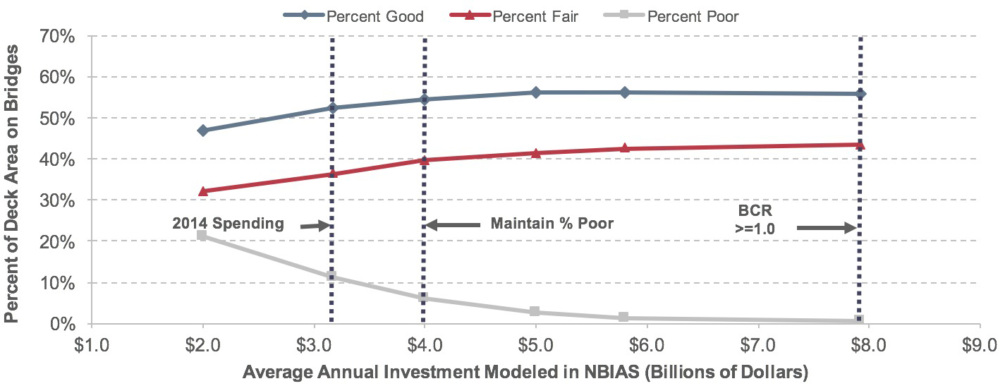
| NBIAS-Modeled Investment on Interstate Bridges | Projected 2034 Condition Indicators—Interstate Bridges | Link to Chapter 7 Scenario | ||||
|---|---|---|---|---|---|---|
| Average Annual Investment (Billions of 2014 Dollars)1 | Weighted by Deck Area | Health Index | Economic Investment Backlog (Billions of 2014 Dollars)1 | |||
| Percent Good | Percent Fair | Percent Poor | ||||
| $7.9 | 55.8% | 43.6% | 0.6% | 95.3 | $0.0 | BCR >= 1.0 |
| $5.8 | 56.0% | 42.6% | 1.4% | 95.3 | $0.7 | |
| $5.0 | 56.1% | 41.3% | 2.6% | 95.1 | $5.9 | |
| $4.0 | 54.5% | 39.6% | 5.9% | 93.7 | $20.4 | Maintain % Poor |
| $3.2 | 52.4% | 36.4% | 11.2% | 91.3 | $36.8 | 2014 Spending |
| $2.0 | 46.9% | 32.1% | 21.0% | 86.2 | $66.6 | |
| Base Year Values: | 36.5% | 57.5% | 5.9% | 91.7 | $36.6 | |
1 The amounts shown do not reflect system expansion needs; the bridge components of such needs are addressed as part of the HERS model analysis.
Source: National Bridge Investment Analysis System.
Key Takeaways
- The 2014 level of investment in service expansion ($6.4 billion) is sufficient to accommodate an average annual ridership increase of 1.3 percent, smaller than the 15-year historical rate of 1.5 percent. This might result in more crowded conditions in stations, trains, and buses, and reduced operating speeds.
- However, the 2014 investment levels are sufficient to accommodate the low ridership growth scenario (1.3 percent). If ridership grows at the 1.3–1.8-percent range (± 0.3 percent around the 15-year historical growth rate), investment in expansion in the $6.0 billion–$8.0 billion range would be needed to avoid deterioration of service quality.
Impacts of Transit Investment
This section examines how different types and levels of annual capital investments would likely affect transit system condition and performance by 2034. It begins with an overview of the types of capital spending projected by the Federal Transit Administration’s (FTA’s) Transit Economic Requirements Model (TERM), the primary analysis tool used to assess transit investment needs and impacts in Part II of this report. The section then examines how variations in the level of annual capital spending are likely to affect future transit conditions and performance.
Impacts of Systemwide Investments Modeled by TERM
This section uses TERM analyses to assess how various levels of investment in the preservation and expansion of the Nation’s transit asset base can be expected to influence transit conditions and performance over the next 20 years. A key objective here is to place a broad range of potential future investment levels—and the consequences of those levels of investment—within the context of both the current expenditures on transit preservation and expansion and some potential investment goals (e.g., attainment of an SGR within 20 years). More specifically, these analyses consider the impact of different levels of transit capital expenditures on the following:
- Preservation Investments—Average condition rating of U.S. transit assets and SGR backlog
- Expansion Investments—Additional ridership (boardings) capacity
Impact of Preservation Investments on Transit Backlog and Conditions
This subsection considers the expected impact of varying levels of aggregate capital reinvestment by all levels of government on the future investment backlog and physical condition (as of 2034) for the Nation’s existing stock of transit assets.
Transit Backlog
The 2010 Conditions and Performance Report introduced the concept of reinvestment backlog as an indication of the amount of near-term investment that would be needed to replace assets that are beyond their expected useful lifetime. Reinvestment backlog focuses attention on assets that are in the worst condition rather than on the average condition of all assets, which is reported in Exhibit 10-19 and had been the primary measure in previous editions. This additional perspective is needed because average condition has become less meaningful in the current environment as an indicator of the health of the current system, with high levels of investment in new assets for transit system expansion raising the systemwide averages independent of the state of existing transit assets. Reinvestment backlog is a measure of the potential need for investment in infrastructure preservation. TERM estimates that reinvestment backlog is $98.0 billion (see Chapter 7).
Exhibit 10-19: Impact of Preservation Investment on 2034 Transit State of Good Repair Backlog in All Urbanized and Rural Areas1
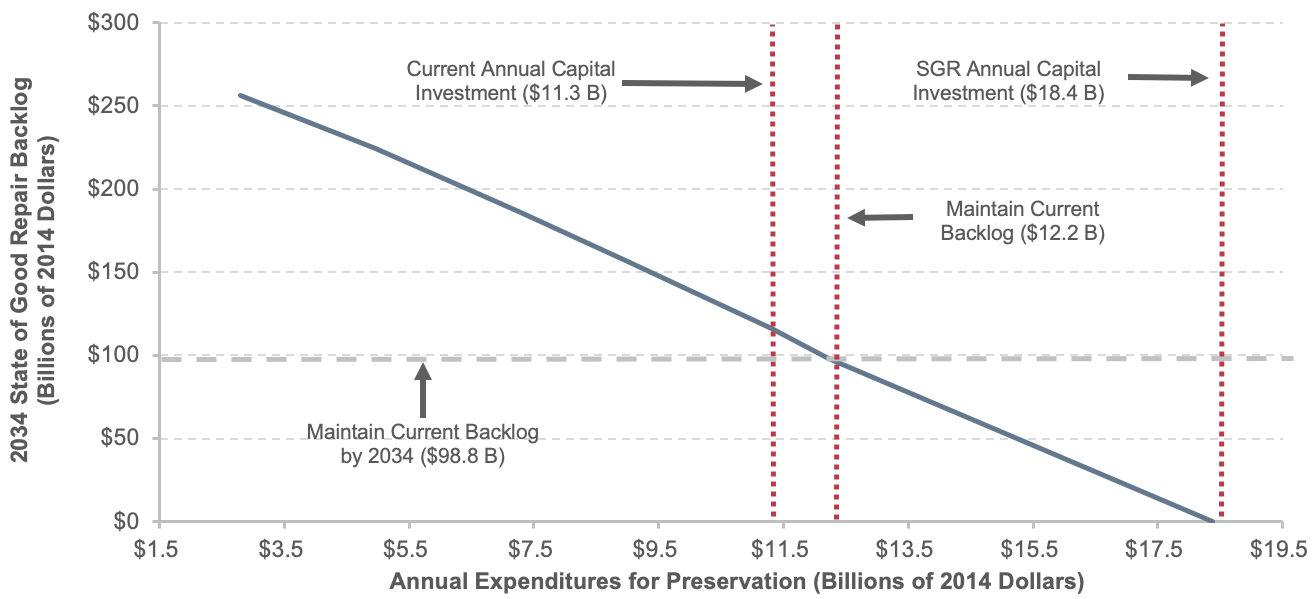
| Average Annual Investment (Billions of 2014 Dollars) | Average Annual Percent Change vs. 2014 | Average Condition Rating in 2034 | Backlog in 2034 (Billions of 2014 Dollars) | Percent Change From Current Backlog | Funding Level Description |
|---|---|---|---|---|---|
| $18.4 | 4.6% | 3.01 | $0.0 | -100% | SGR (Unconstrained, Replace at 2.50) |
| $12.2 | 0.8% | 2.85 | $98.0 | 0% | Maintain Current Backlog |
| $11.3 | 0.0% | 2.81 | $116.2 | 19% | 2014 Capital Expenditures (Sustain 2014 Spending) |
| $9.0 | -2.4% | 2.72 | $157.1 | 60% | |
| $7.2 | -4.8% | 2.63 | $186.6 | 90% | |
| $5.0 | -9.4% | 2.51 | $224.3 | 129% | |
| $2.8 | -19.0% | 2.43 | $256.5 | 162% |
1 Note that for this report, assets are considered past their useful lives once their estimated condition in TERM falls below condition 2.50.
Source: Transit Economic Requirements Model.
Exhibit 10-19 focuses on the impact of future spending levels on this reinvestment backlog. Specifically, Exhibit 10-19 presents the estimated impact of differing levels of annual capital reinvestment on the expected size of the reinvestment backlog in 2034. Here the reinvestment backlog is defined as the level of investment required to bring all of the Nation’s assets to an SGR. This includes replacing those assets that currently exceed their useful lives (the $98.0 billion) and completing all major rehabilitation activities and replacing assets that will exceed their useful lives during the analysis period. If future reinvestment rates are insufficient to address these ongoing reinvestment needs as they arise, the size of the backlog will increase over time. Reinvestment at a rate above that required to address new needs as they arise will ultimately result in elimination of the existing backlog.
As shown in Exhibit 10-19, TERM analysis suggests that the current rate of capital reinvestment of $11.3 billion is insufficient to keep pace with ongoing rehabilitation and replacement needs and, if maintained over the next 20 years, would result in a reinvestment backlog of roughly $116.2 billion by 2034. In contrast, increasing the annual rate of reinvestment to an average of $18.4 billion would eliminate the backlog by 2034. The annual level of reinvestment would need to be increased to roughly $12.2 billion just to maintain the backlog at roughly its current size.
Transit Conditions
Exhibit 10-20 presents the estimated impact of various levels of annual rehabilitation and replacement investments on the average physical condition of all existing assets nationwide as of 2034. The exhibit shows ongoing improvements to the overall condition of the Nation’s existing transit asset base from increasing levels of transit capital reinvestment. Of special note is that average condition provides a measure of asset conditions taken together. Hence, despite the fact that overall conditions improve with additional expenditures, the condition of some individual assets is expected to continue to deteriorate (given the length of asset lives and the timing of their replacement cycles) while the condition of other assets improves. The value of the aggregate measure lies in providing an overall, single measure of asset conditions. Moreover, given the relationship between asset condition and asset reliability, any general improvement in overall asset conditions also can be associated with related improvements to service quality and reliability.
The table portion of Exhibit 10-20 presents the same investment and average condition information as in the chart. This table also presents the impact of reinvestment on asset conditions for five key transit asset categories (i.e., guideway and track, facilities, systems, stations, and vehicles) and the average annual percentage change in constant dollar funding from 2014 levels to achieve each projected condition level.
Further review of Exhibit 10-20 reveals several observations: First, almost none of the selected reinvestment rates presented (including the 2014 level of reinvestment, which was $11.3 billion) is sufficient to maintain aggregate conditions at or near the current national average condition rating of 3.1. Only the highest reinvestment rate presented here of $21.8 billion annually (replacement at condition rating 3.0), which is an aggressive reinvestment rate, is sufficient to maintain aggregate conditions at current levels. A primary factor driving this result is the ongoing expansion investment in new rail systems over the past several decades. Although this expansion investment has tended to maintain or even increase the average condition rating of assets nationwide (despite the ongoing deterioration of older assets), it also has resulted in an average condition rating that is not sustainable in the long term (i.e., without including the influence of further expansion investments or replacing assets at an unreasonably early age).
Second, reinvestment at roughly $18.4 billion annually is required to attain an SGR condition by 2034, and this level of reinvestment is estimated to yield an average condition value of roughly 3.01 by that year. Given the definition of the SGR benchmark (described in more detail in Chapter 7), which seeks to eliminate the existing investment backlog and then address all subsequent rehabilitation and replacement activities “on time” thereafter, the 3.01 value could be considered representative of the expected long-term average condition of a well-maintained and financially and economically unconstrained national transit system. Hence, an average condition rating of roughly 3.01 represents a more reasonable long-term condition target for existing transit infrastructure than the current aggregate rating of 3.1.
Exhibit 10-20: Impact of Preservation Investment on 2034 Transit Conditions in All Urbanized and Rural Areas
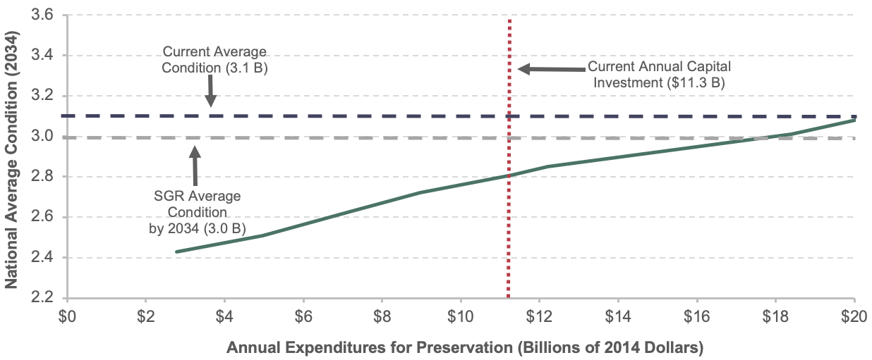
| Average Annual Investment (Billions of 2014 Dollars) Total Capital Outlay | Average Annual Percent Change vs. 2014 | Average Transit Conditions in 2034 | Notes | |||||
|---|---|---|---|---|---|---|---|---|
| Asset Categories | All Transit Assets | |||||||
| Guideway | Facilities | Systems | Stations | Vehicles | ||||
| $21.8 | 6.1% | 2.75 | 3.33 | 3.83 | 2.99 | 3.53 | 3.12 | Unconstrained, Replace at 3.00 |
| $20.0 | 5.4% | 2.73 | 3.33 | 3.70 | 2.99 | 3.47 | 3.08 | Unconstrained, Replace at 2.75 |
| $18.4 | 4.6% | 2.69 | 3.28 | 3.58 | 2.97 | 3.33 | 3.01 | SGR (Unconstrained, Replace at 2.50) |
| $12.2 | 0.8% | 2.63 | 2.68 | 3.52 | 2.46 | 3.25 | 2.85 | Maintain Current Backlog |
| $11.3 | 0.0% | 2.61 | 2.68 | 3.40 | 2.33 | 3.25 | 2.81 | 2014 Capital Expenditures |
| $9.0 | -2.4% | 2.47 | 2.68 | 3.30 | 2.31 | 3.25 | 2.72 | |
| $7.2 | -4.8% | 2.43 | 2.68 | 3.00 | 2.24 | 3.21 | 2.63 | |
| $5.0 | -9.4% | 2.36 | 2.68 | 2.64 | 2.22 | 3.03 | 2.51 | |
| $2.8 | -19.0% | 2.32 | 2.68 | 2.56 | 2.21 | 2.70 | 2.43 | |
1 Note that the conditions of individual transit assets are estimated using TERM’s asset decay curves, which estimate asset conditions on a scale of 5 (excellent) through 1 (poor), as described earlier in this chapter and in Appendix C of this report. The average national condition is the weighted average of the condition of all assets nationwide, weighted by the estimated replacement cost of each asset.
2 Note that this preservation analysis is intended to consider reinvestment needs only for existing transit assets (as of 2014), not for expansion assets to be added to the existing capital stock in future years.
Source: Transit Economic Requirements Model.
Another observation is that a significant level of reinvestment is required to alter the estimated 2034 average condition measure by a point or more. This result is also driven in part by a large proportion of transit assets with expected useful lives of 80 years or more that will not require significant reinvestment over the 20-year period of this analysis (regardless of the level of reinvestment). These assets tend to contribute a high weighting in the average condition measure, making the measure somewhat insensitive to the rate of reinvestment (note that a high proportion of reinvestment activity is focused on the replacement of those assets with relatively shorter useful lives, such as vehicles).
Finally, TERM prioritizes asset needs based on five criteria (condition, reliability, safety, riders impacted, and operations and maintenance cost impacts) with condition having the highest weighting. Replacement and rehabilitation investments are both subject to this same prioritization scoring. Replacement needs tend to score higher, however, as they tend to reflect the needs of assets that are in poorer condition than those assets requiring rehabilitation. Therefore, rehabilitation needs tend not to be addressed until most (but far from all) replacement needs are addressed. TERM currently predicts improvement in asset condition only following a replacement. Thus, expenditures beyond approximately $11.8 billion on the chart increase total cost as rehabilitation projects are added, but these projects do not contribute to an increase in condition.
Impact of Expansion Investments on Transit Ridership
Although capital spending on preservation primarily benefits the physical condition of existing transit assets, expansion investments are typically undertaken to expand the asset base to accommodate projected growth in ridership and potentially to improve service performance for existing transit system users.
Exhibit 10-21 shows the relationship between aggregated annual capital spending by all levels of government on expansion investments and the additional number of annual passenger boardings that transit systems would be able to support by 2034. More precisely, this chart presents the level of expansion investment required to ensure that transit vehicle occupancy rates are maintained at current levels over the next two decades for a broad range of the potential rates of growth in transit passenger miles traveled. As the upward sloping curve of the chart indicates, higher levels of investment are required to support greater numbers of additional riders at a constant level of service. If investment levels are insufficient to support the projected growth in ridership fully, vehicle occupancy rates will tend to increase, leading to increased crowding on high-utilization systems and potentially leading to increased dwell times at stops, reduced average operating speeds, and increased rates of vehicle wear. Conversely, if the rate of transit capacity expansion exceeds the actual rate of ridership growth, occupancy rates will tend to decline, but cost-effectiveness (operating expenses per PMT) and other financial indicators will worsen, increasing the operating deficit which might require fare increases and/or additional State, local, or Federal assistance.
The findings presented in Exhibit 10-21 suggest the following trends. First, the 2014 rate of investment in asset expansion ($6.4 billion in 2014 dollars) could support roughly 3.3 billion additional boardings by 2034 (approximately a 1.3-percent annual growth in ridership). If the actual rate of future ridership growth is close to the trend rate of growth for the past 15 years, an average capital investment of $7.0 billion annually in transit expansion would be required over the next 20 years to support an additional 3.7 billion annual boardings—again after excluding expansion investments that do not pass TERM’s benefit-cost test. Thus, the 2014 level of transit capital expansion investment is close to—but somewhat less than—that required to support future rider growth, assuming future growth aligns with the 15-year historical trend. The end result would be increased crowding on some bus and rail systems, increased rates of asset wear, and the potential for increased service delays due to crowding, dwell time increases, and breakdowns.
Exhibit 10-21: New Ridership Supported in 2034 by Expansion Investments in All Urbanized and Rural Areas 1
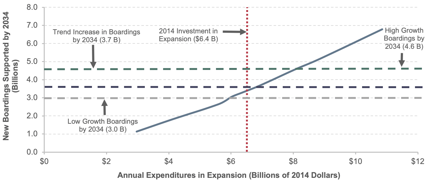
| Total New Boardings by 2034 | ||||
|---|---|---|---|---|
| Average Annual Investment (Billions of 2014 Dollars) | Average Annual Percent Change vs. 2010-2014 Average | New Riders Supported (Billions of Annual Boardings) | Average Annual Growth in Boardings1 | Funding Level Description |
| $10.9 | 5.0% | 6.8 | 2.5% | Highest Growth Scenario (+1.0%) |
| $8.9 | 3.2% | 5.2 | 2.0% | Higher Growth Scenario (+0.5%) |
| $8.1 | 2.3% | 4.6 | 1.8% | High Growth Scenario (+0.3%) |
| $7.0 | 0.9% | 3.7 | 1.5% | 15 Year Historic Growth Rate Trend |
| $6.4 | 0.0% | 3.3 | 1.3% | 2014 Capital Expenditures |
| $6.4 | -0.6% | 3.0 | 1.3% | Low Growth Scenario (-0.3%) |
| $5.6 | -1.3% | 2.6 | 1.1% | Lower Growth Scenario (-0.5%) |
| $4.1 | -4.6% | 1.8 | 0.8% | Lower Growth Scenario (-1.0%) |
| $3.0 | -8.7% | 1.1 | 0.5% | Lowest Growth Scenario (-1.5%) |
1 As compared with total urban ridership in 2014; only includes increases covered by investments passing TERM's benefit-cost test.
Note: TERM assesses expansion needs at the agency-mode level subject to (1) current vehicle occupancy rates at the agency-mode level and (2) expected transit PMT growth at the UZA level (hence, all agency modes within a given UZA are subject to the same transit PMT growth rate). However, TERM does not generate expansion needs estimates for agency modes that have occupancy rates that are well below the national average for that mode.
Source: Transit Economic Requirements Model.