

This edition of the C&P Report is based primarily on data through 2014. In assessing recent trends, this report generally focuses on the 10-year period from 2004 to 2014. The prospective analyses generally cover the 20 year period ending in 2034; the investment levels associated with these scenarios are stated in constant 2014 dollars. This section presents key findings for the overall report; key findings for individual chapters are presented in the Executive Summary.
Highlights: Highways and Bridges
Extent of the System
Highway System Terminology
“Federal-aid highways” are roads that generally are eligible for Federal funding assistance under current law. (Note that certain Federal programs do allow the use of Federal funds on other roadways.)
The “National Highway System” (NHS) includes those roads that are most important to interstate travel, economic expansion, and national defense. It includes the entire Interstate System. The NHS was expanded under MAP-21.
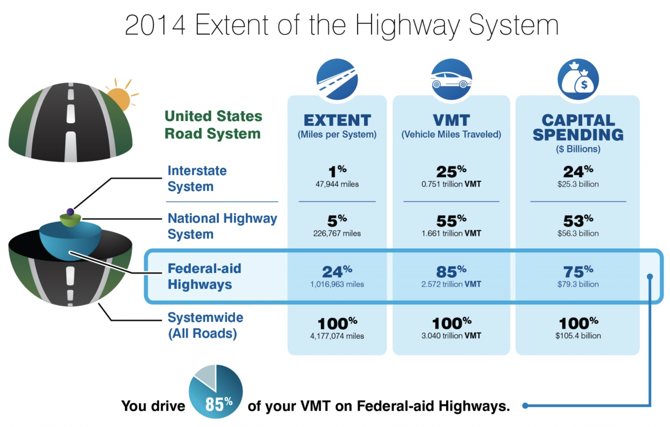
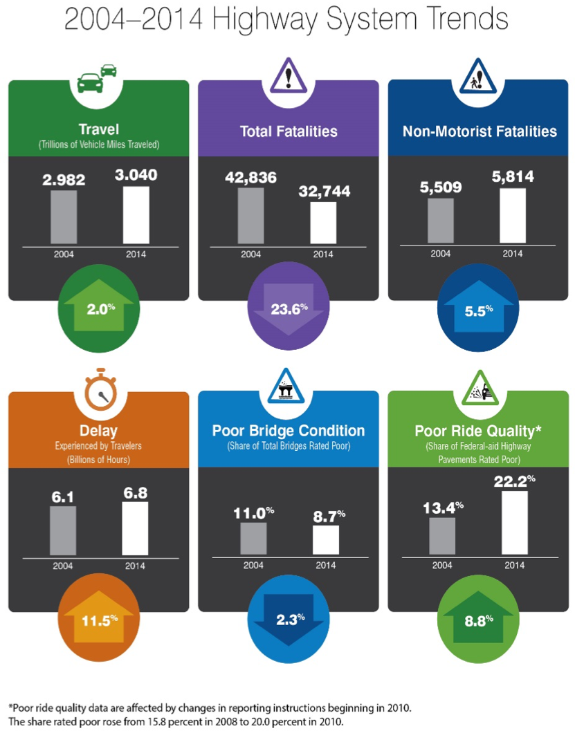
- The Nation’s road network included 4,177,074 miles of public roadways and 610,749 bridges in 2014. This network carried more than 3.040 trillion vehicle miles traveled (VMT) and almost 5.205 trillion person miles traveled, up from 2.982 trillion VMT and up from 4.876 trillion person miles traveled in 2004.
- The 1,016,963 miles of Federal-aid highways (24 percent of total mileage) carried 2.572 trillion VMT (85 percent of total travel) in 2014.
- Although the 226,767 miles on the National Highway System (NHS) comprise only 5 percent of total mileage, the NHS carried 1.661 trillion VMT in 2014, approximately 55 percent of total travel.
- The 47,944 miles on the Interstate System carried 0.751 trillion VMT in 2014, slightly over 1 percent of total mileage and just under 25 percent of total VMT. The Interstate System has grown since 2004, when it consisted of 46,836 miles carrying 0.727 trillion VMT
Spending on the System
- All levels of government spent a combined $222.6 billion for highway-related purposes in 2014. About 47.4 percent of total highway spending ($105.4 billion) was for capital improvements to highways and bridges; the remainder included expenditures for physical maintenance, highway and traffic services, administration, highway safety, and debt service.
- Of the $105.4 billion spent on highway capital improvements in 2014, $25.3 billion (24 percent) was spent on the Interstate System, $56.3 billion (53 percent) was spent on the NHS, and $79.3 billion (75 percent) was spent on Federal-aid highways (including the NHS)
- In nominal dollar terms, highway spending increased by 50.9 percent (4.2 percent per year) from 2004 to 2014; after adjusting for inflation, this equates to a 9.5-percent increase (0.9 percent per year).
- Highway capital expenditures rose from $70.3 billion in 2004 to $105.4 billion in 2014, a 50.0-percent (4.1 percent per year) increase in nominal dollar terms; after adjusting for inflation, this equates to a 1.0 percent (0.1 percent per year) decrease, meaning that capital spending did not keep pace with increases in construction costs.
Constant-Dollar Conversions for Highway Expenditures
This report uses the Federal Highway Administration’s National Highway Construction Cost Index (NHCCI) 2.0 for inflation adjustments to highway capital expenditures and the Consumer Price Index (CPI) for adjustments to other types of highway expenditures. From 2004 to 2014 the NHCCI 2.0 increased by 51.5 percent (4.2 percent per year), while the CPI increased by only 25.3 percent (2.3 percent per year). Previous editions of the C&P Report reflected an earlier version of the NHCCI, which showed smaller increases than the CPI in recent years.
- The portion of total highway capital spending funded by the Federal government decreased from 43.8 percent in 2004 to 42.5 percent in 2014. Federally funded highway capital outlay grew by 3.8 percent per year over this period, compared with a 4.4-percent annual increase in capital spending funded by State and local governments.
- The composition of highway capital spending shifted from 2004 to 2014. The percentage of highway capital spending directed toward system rehabilitation rose from 51.7 percent in 2004 to 62.0 percent in 2014. Over the same period, the percentage of spending directed toward system enhancement rose from 11.2 percent to 13.5 percent, while the percentage of spending directed toward system expansion fell from 37.1 percent to 24.5 percent.
Highway Capital Spending Terminology
This report splits highway capital spending into three broad categories. “System rehabilitation” includes resurfacing, rehabilitation, or reconstruction of existing highway lanes and bridges. “System expansion” includes the construction of new highways and bridges and the addition of lanes to existing highways. “System enhancement” includes safety enhancements, traffic control facilities, and environmental enhancements.
Conditions and Performance of the System
Highway vehicle miles traveled increased by 2.0 percent (0.2 percent per year) from 2004 to 2014, while highway capital spending declined by 1.0 percent in constant-dollar terms (and overall highway spending increased). These trends were present while indicators of the performance and condition of the overall system had mixed results.
Pavement Condition Trends Have Been Mixed
Pavement Condition Terminology
This report uses the International Roughness Index (IRI) as a proxy for overall pavement condition. Pavements with an IRI value of less than 95 inches per mile are considered to have “good” ride quality. Pavements with an IRI value greater than 170 inches per mile are considered to have “poor” ride quality. Pavements that fall between these two ranges are considered “fair.”
- In general, pavement condition trends over the past decade have been better on the NHS (the 5 percent of total system mileage that carries 55 percent of total system VMT) than on Federal-aid highways (the 24 percent of system mileage that carries 85 percent of total system VMT, including the NHS).
- The share of Federal-aid highway VMT on pavements with “good” ride quality rose from 44.2 percent in 2004 to 47.0 percent in 2014. The share of mileage with good ride quality declined from 43.1 percent to 38.4 percent over this same period, however, indicating that conditions have worsened on roads with lower travel volumes.
- The share of Federal-aid highway pavements with “poor” ride quality rose from 2004 to 2014, as measured on both a VMT-weighted basis (rising from 15.1 percent to 17.3 percent) and a mileage basis (rising from 13.4 percent to 22.2 percent). Although this trend is exaggerated due to changes in data reporting instructions beginning in 2010, the data clearly show that more of the Nation’s pavements have deteriorated to the point that they are adding to vehicle operating costs and reducing driver comfort.
- The share of VMT on NHS pavements with good ride quality rose from 52 percent in 2004 to 59 percent in 2014. This gain is especially impressive considering MAP-21 expanded the NHS by 62,292 miles (37 percent), as pavement conditions on the additions to the NHS were not as good as those on the pre-expansion NHS. The share rose from 52 percent in 2004 to 60 percent in 2010 based on the pre-expansion NHS and from an estimated 54.7 percent in 2010 to 58.7 percent in 2014 based on the post-expansion NHS, which translates into an average increase of more than 1 percentage point per year.
- The share of VMT on NHS pavements with poor ride quality declined from 9 percent to 7 percent from 2004 to 2010; since the expansion of the NHS under MAP-21, this share has remained relatively constant at approximately 11 percent.
FHWA Bridge Classifications
FHWA is currently transitioning to a new set of bridge condition descriptors. Bridges are given an overall rating of “poor” if the deck, substructure, or superstructure is found to be in poor condition due to deterioration or damage. The legacy term “structurally deficient” includes “poor” bridges as well as those failing other criteria, such as adequacy of the waterway opening under the bridge. The classification of a bridge as poor or structurally deficient does not mean it is unsafe.
These classifications are often weighted by bridge deck area, recognizing that bridges are not all the same size and, in general, larger bridges are more costly to rehabilitate or replace to address deficiencies. The classifications are also sometimes weighted by annual daily traffic, recognizing that more heavily traveled bridges have a greater impact on total highway user costs.
Another legacy term is “functionally obsolete,” which relates to the geometric characteristics of a bridge (e.g., bridge width, load-carrying capacity, clearances, approach roadway alignment) in relation to current design standards. The magnitude of such deficiencies determines whether a bridge is classified as “functionally obsolete.” This metric is a legacy classification that was used to implement the Highway Bridge Program, which was discontinued as a separate program with the enactment of MAP-21. In the absence of a programmatic reason to collect the data necessary to support this classification, some of the data necessary to compute it are being removed from the National Bridge Inventory. Future editions of the C&P Report will not contain this information. This edition presents “functionally obsolete” as a measure of operational performance, rather than a measure of physical conditions.
Bridge Condition Trends Have
Been Mixed
- Based directly on bridge counts, the share of bridges classified as poor has improved, dropping from 11.0 percent in 2004 to 8.7 percent in 2014 (and to 8.3 percent in 2015). The share of NHS bridges classified as poor also improved over this period, dropping from 5.6 percent to 4.1 percent (and to 3.7 percent in 2015).
- Weighted by deck area, the share of bridges classified as poor improved, declining from 9.4 percent in 2004 to 6.7 percent in 2014 (and to 6.4 percent in 2015). The deck area-weighted share of poor NHS bridges dropped from 8.7 percent to 5.8 percent over this period (and to 5.5 percent in 2015).
- Weighted by deck area, the share of bridges classified as structurally deficient improved, declining from 10.1 percent in 2004 to 7.1 percent in 2014. The deck area-weighted share of structurally deficient NHS bridges dropped from 8.9 percent to 6.0 percent over this period.
- While the percentage of poor bridges has declined over the last decade, the share of bridges classified as good has also gone down. Weighted by deck area, the share of bridges classified as good worsened, declining from 46.1 percent in 2004 to 44.7 percent in 2014 (before rebounding to 45.5 percent in 2015). The deck area-weighted share of good NHS bridges dropped from 43.8 percent to 42.2 percent over this period (rising to 43.0 percent in 2015).
Operational Performance in Urbanized Areas Has Slowly Worsened
- The Texas Transportation Institute 2015 Urban Mobility Scorecard estimates that the average commuter in 471 urbanized areas experienced a total of 42 hours of delay resulting from congestion in 2014, up from 41 hours in 2004. Congestion delay was worse in the largest metro areas, for example averaging 82 hours in Washington D.C., 80 hours in Los Angeles/Long Beach, 78 hours in San Francisco/Oakland, and 74 hours in New York/Newark. Total delay experienced by all urbanized area travelers combined rose by 11.5 percent from 6.1 billion hours in 2004 to 6.8 billion hours in 2014, an all-time high.
- The combined cost of wasted time and wasted fuel caused by congestion in urbanized areas rose from an estimated $136 billion in 2004 to $160 billion in 2014. Although these costs had declined during the most recent recession, they now exceed their pre-recession peak.
- One indicator with more positive trends relates to bridge geometrics, which can influence operational performance. Based directly on bridge counts, the share of bridges classified as functionally obsolete declined from 15.2 percent in 2004 to 13.8 percent in 2014 (unchanged at 13.8 percent in 2015). Weighted by deck area, the share of bridges classified as functionally obsolete improved slightly, dropping from 20.5 percent in 2004 to 20.3 percent in 2014 (before rebounding to 20.5 percent in 2015). Functional obsolescence tends to be a more significant problem on larger bridges carrying more traffic.
Highway Safety Improved Overall, but Nonmotorist Fatalities Rose
- The annual number of highway fatalities was reduced by 23.6 percent from 2004 to 2014, dropping from 42,836 to 32,744 (before rising to 35,485 in 2015 and 37,806 in 2016, then declining to 37,133 in 2017).
- From 2004 to 2014, the number of nonmotorists (pedestrians, bicyclists, etc.) killed by motor vehicles increased by 5.5 percent, from 5,509 to 5,814 (17.8 percent of all fatalities). From 2006 to 2009, nonmotorist fatalities showed a steady decline of 15.0 percent, but beginning in 2009 that trend began to shift and resulted in a 19.6-percent increase through 2014. (Nonmotorist fatalities rose to 6,556 in 2015 and 7,193 in 2016 before declining to 6,988 in 2017).
- Fatalities related to roadway departure decreased by 24.8 percent from 2004 to 2014, but roadway departure remains a factor in over half (54.4 percent) of all highway fatalities. Intersection-related fatalities decreased by 17.0 percent from 2004 to 2014, but over one-fourth (26.5 percent) of highway fatalities in 2014 occurred at intersections.
- The fatality rate per 100 million VMT declined from 1.45 in 2004 to an all-time low of 1.08 in 2014 (before rising to 1.15 in 2015 and 1.19 in 2016, then declining to 1.16 in 2017).
- The number of traffic-related injuries decreased by 18.8 percent, from 2.7 million in 2004 to 2.2 million in 2014. The injury rate per 100 million VMT declined from 90 in 200 to 71 in 2014.
Future Capital Investment Scenarios
The scenarios that follow pertain to spending by all levels of government combined for the 20-year period from 2014 to 2034 (reflecting the impacts of spending from 2015 through 2034); the funding levels associated with all of these analyses are stated in constant 2014 dollars. The results below apply to the overall road system; separate analyses for the Interstate System, the NHS, and Federal-aid highways are presented in the body of this report.
Modeled vs. Nonmodeled Investment
Each highway investment scenario includes projections for system conditions and performance based on simulations using the Highway Economic Requirements System (HERS) and National Bridge Investment Analysis System (NBIAS). Each scenario scales up the total amount of simulated investment to account for capital improvements that are outside the scopes of the models, or for which no data are available to analyze. In 2014, 13.5 percent of highway capital spending was used for system enhancements (safety enhancements, traffic control facilities, and environmental enhancements) that neither model analyzes directly. An additional 15.8 percent was used in 2014 for pavement and capacity improvements on non-Federal-aid highways; FHWA does not collect the detailed information for such roadways that would be necessary to support analysis using HERS. (FHWA does collect sufficient data for all of the nation’s bridges to support analysis using NBIAS.)
Combining these two percentages yields a total of 29.3 percent; each scenario for the overall road system was scaled up so that nonmodeled investment would comprise this share of its total investment level.
Highway Investment / Performance Analyses
To provide an estimate of the costs that might be required to maintain or improve system performance, this report includes a series of investment/performance analyses that examine the potential impacts of alternative levels of future combined investment by all levels of government on highways and bridges for different subsets of the overall system
Drawing on these investment/performance analyses, a series of illustrative scenarios was selected for more detailed exploration and presentation.
The Sustain 2014 Spending scenario and the Maintain Conditions and Performance scenario each assume a fixed level of highway capital spending in each year in constant-dollar terms (i.e., spending keeps pace with inflation each year).
Spending under the Improve Conditions and Performance scenario varies by year depending on the set of potential cost-beneficial investments available at that time. Because there is an existing backlog of cost-beneficial investments that have not previously been addressed, investment under this scenario is frontloaded, with higher levels of investment in the early years of the analysis and lower levels in the latter years.
Sustain 2014 Spending Scenario
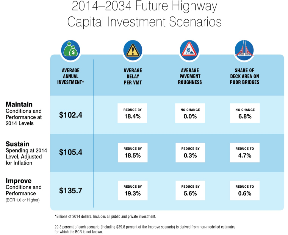
- The Sustain 2014 Spending scenario assumes that capital spending by all levels of government is sustained in constant-dollar terms at the 2014 level ($105.4 billion systemwide) through 2034. It also assumes that spending would be directed toward projects with the largest benefit-cost ratios. At this level of capital investment, average pavement roughness on Federal-aid highways would be projected to improve by 0.3 percent, while the share of bridges classified as poor would be projected to improve, declining from 6.8 percent in 2014 to 4.7 percent in 2034. Average delay per VMT would be projected to improve by 18.5 percent, as travel growth gradually slows over time and various highway management and operational strategies are adopted more broadly.
Maintain Conditions and Performance Scenario
- The Maintain Conditions and Performance scenario seeks to identify a level of capital investment at which selected measures of future conditions and performance in 2034 are maintained at 2014 levels. It also assumes that spending would be directed toward projects with the largest benefit-cost ratios. The average annual level of investment associated with this scenario is $102.4 billion, 2.9 percent less than actual highway capital spending by all levels of government in 2014.
- Under this scenario, $66.5 billion per year would be directed to system rehabilitation, $22.1 billion to system expansion, and 13.8 billion to system enhancement. Average pavement roughness on Federal-aid highways and the share of bridges classified as poor in 2034 would match their 2014 levels. Average delay per VMT would be projected to improve by 18.4 percent, as travel growth gradually slows over time and various highway management and operational strategies are adopted more broadly.
Improve Conditions and Performance Scenario
- The Improve Conditions and Performance scenario seeks to identify the level of capital investment needed to address all potential investments estimated to be cost-beneficial. The average annual level of systemwide capital investment associated with this scenario is $135.7 billion, 28.8 percent higher than actual 2014 capital spending.
- Approximately 29 percent of the investment under the Improve Conditions and Performance scenario would go toward addressing an existing backlog of cost-beneficial investments of $786.4 billion. The rest would address new needs arising from 2015 through 2034.
- The State of Good Repair benchmark represents the subset of the Improve Conditions and Performance scenario spending level that is directed toward addressing deficiencies in the physical condition of existing highway and bridge assets. The average annual investment level associated with this benchmark is $88.4 billion, 65.1 percent of the $135.7 billion cost of the overall scenario. The scenario also includes average annual spending of $29.1 billion (21.4 percent) directed toward system expansion, and $18.3 billion (13.5 percent) directed toward system enhancement.
- An estimated $39.8 billion of the spending in this scenario is not constrained by benefit-cost analysis because it is outside the scope of the models. The amount of such “nonmodeled” spending included in this scenario’s estimate is equal to the share of capital spending in 2014 that was outside the scope of the models. Such spending is for system enhancement projects on all public roads, and pavement rehabilitation and capacity expansion projects on non-Federal aid highways.
- Under the Improve Conditions and Performance scenario, average pavement roughness on Federal-aid highways would be projected to improve by 5.6 percent, while the share of bridges classified as poor would be projected to improve, declining from 6.8 percent in 2014 to 0.6 percent in 2034. This scenario would not eliminate all poor pavements and bridges because, while in some cases it is cost-beneficial to proactively improve assets before they become poor, in other cases it only becomes cost-beneficial to improve assets after they have declined into poor condition. Therefore, at the end of any given year, some portion of the pavement and bridge population would remain deficient.
Highlights: Transit
Extent of the System
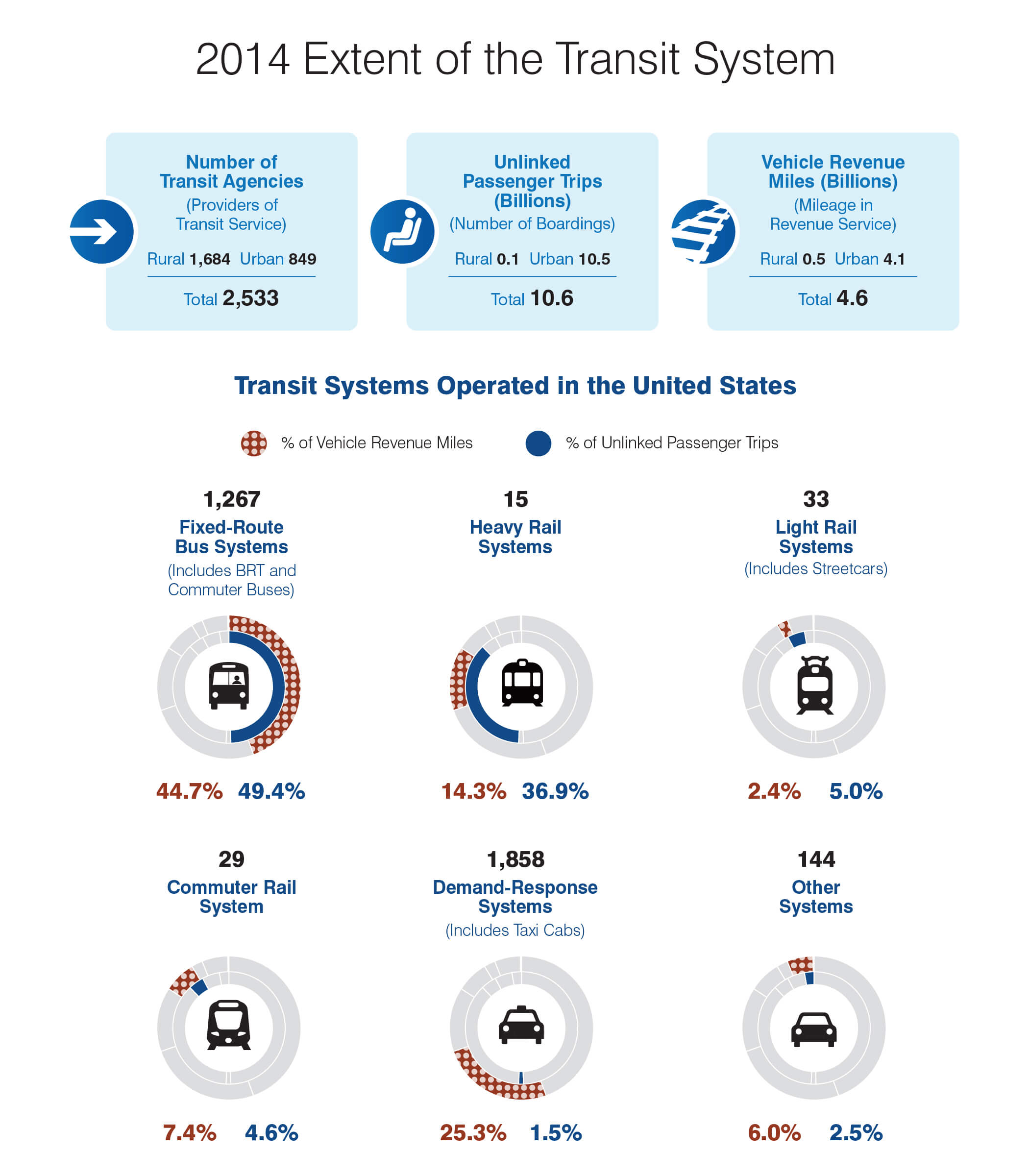
- Of the transit agencies that submitted data to the National Transit Database (NTD) in 2014, 849 provided service primarily to urbanized areas and 1,684 provided service to rural areas. Urban and rural agencies operated 1,267 bus systems, 1,858 demand-response systems, 15 heavy rail systems, 29 commuter rail systems, 33 light rail and streetcar systems, 25 streetcar systems, and 5 hybrid rail systems. There were also 98 transit vanpool systems, 29 ferryboat systems, 5 trolleybus systems, 6 monorail and automated guideway systems, 3 inclined plane systems, 1 cable car system, 2 tramway systems, and 1 público. (Público is a mode that exists only in Puerto Rico but has the same operating characteristics as Jitney. These modes operate on fixed routes but with no fixed schedules.)
- Transit operators reported 10.6 billion unlinked passenger trips on 4.6 billion vehicle revenue miles in 2014.
Bus, Rail, and Demand Response: Transit Modes
Public transportation is provided by several different types of vehicles that are used in different operational modes. The most common is fixed-route bus service, which uses different sizes of rubber-tired buses that run on scheduled routes. Commuter bus service is similar, but uses over-the-road buses and runs longer distances between stops. Bus rapid transit is high-frequency bus service that emulates light rail service. Públicos and jitneys are small owner-operated buses or vans that operate on less-formal schedules along regular routes.
Larger urban areas are often served by one or more varieties of fixed-guideway (rail) service. These include heavy rail (often running in subway tunnels), which is primarily characterized by third-rail electric power and exclusive dedicated guideway. Extended urban areas may have commuter rail, which often shares track with freight trains and often uses overhead electric power (but may also use diesel power or third rail). Light rail systems are common in large-and medium-sized urban areas; they feature overhead electric power and run on track that is entirely or in part on city streets that are shared with pedestrian and automobile traffic. Streetcars are small light rail systems, usually with only one or two cars per train that often run in mixed traffic. Hybrid Rail, previously reported as light rail or commuter rail, is a mode with shared characteristics of these two modes. It has higher average station density (stations per track mileage) than commuter rail and lower than light rail; it has a smaller peak-to-base ratio than that of commuter rail. Cable cars, trolley buses, monorail, and automated guideway systems are less-common fixed-guideway systems.
Demand-response transit service is usually provided by vans, taxicabs, or small buses that are dispatched to pick up passengers upon request. This mode is mostly used to provide paratransit service as required by the Americans with Disabilities Act. These vehicles do not follow a fixed schedule or route.
- Bus and heavy rail modes continue to be the largest segments of the industry, serving 48 percent and 37 percent of all transit trips, respectively. Commuter rail supports a relatively high share of passenger miles (20.5 percent). Light rail is the fastest-growing rail mode (with passenger miles growing at 4.7 percent per year between 2004 and 2014), but it still provides only 4.4 percent of transit passenger miles. Vanpool growth during that period was 11.1 percent per year, but with vanpools still accounting for only 2.3 percent of all transit passenger miles.
Federal Transit Funding Urban and Rural
Federal Transit Administration (FTA) Urbanized Area Formula Funds are apportioned to urbanized areas (UZAs), as defined by the Census Bureau. UZAs in this report were defined by the 2010 census. Each UZA has a designated recipient, usually a metropolitan planning organization (MPO) or large transit agency, which then sub-allocates FTA funds in its area according to local policy. The designated recipient may then allow these organizations to apply directly for a grant with FTA as a designated recipient. In small urban and rural areas, FTA apportions funds to the State, which allocates them according to State policy. Indian tribes are apportioned their formula funds directly. Once obligated in a grant, all funds then become available, on a reimbursement basis.
Spending on the System
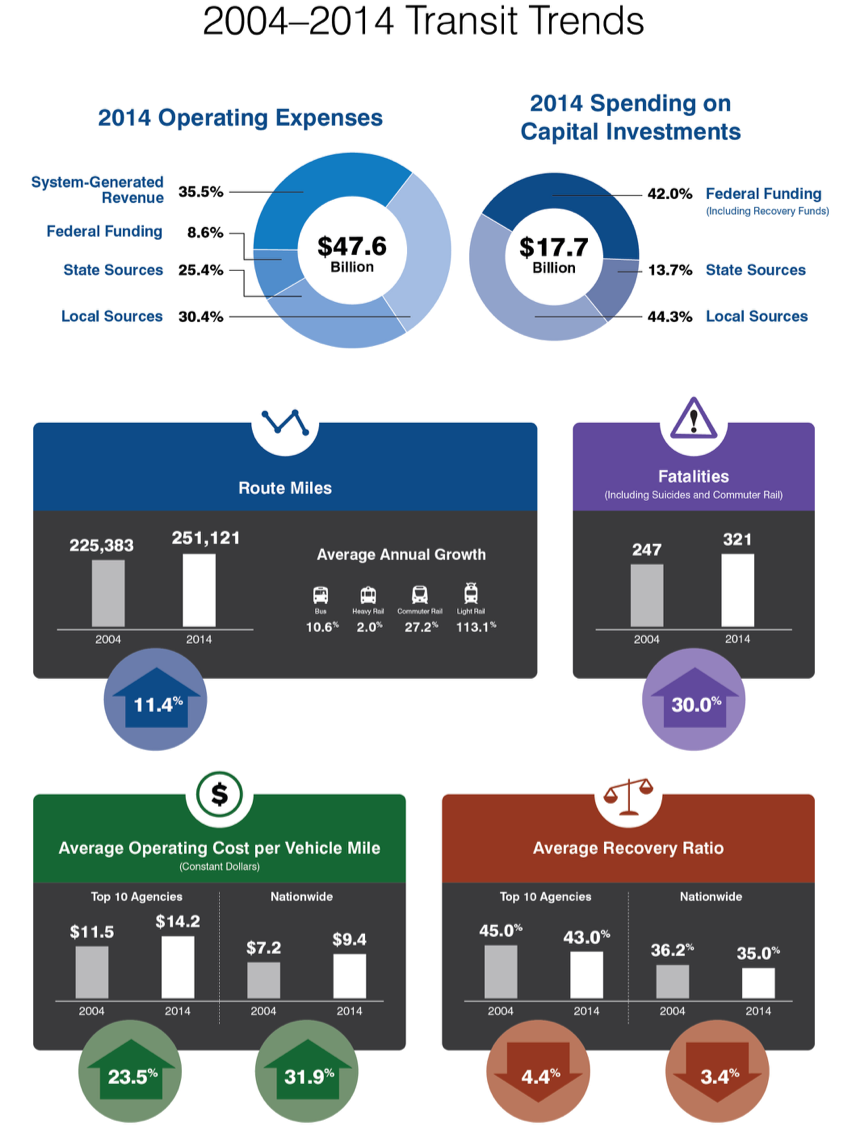
- All levels of government spent a combined $65.2 billion to provide public transportation and maintain transit infrastructure. Of this total, 29 percent was system-generated revenue, of which most came from passenger fares. Eighteen percent of revenues came from the Federal government while the remaining funds came from State and local sources.
- Of the combined $65.2 billion spent on public transportation, public transit agencies spent $17.7 billion on capital investments in 2014. Regularly authorized and appropriated Federal funding made up 39.5 percent of these capital expenditures. Funds from the Federal American Recovery and Reinvestment Act provided another 2.5 percent.
- Federal funding is targeted primarily for capital assistance, although Federal funding for operating expenses at public transportation agencies increased from 30 percent of all Federal funding in 2004 to 36 percent in 2014. Virtually all of the increase is due to increased use of “preventive maintenance” eligible for reimbursement from 5307 grant funds
- From 2004 to 2014, the urban systems’ total fares per revenue mile increased by 1.6 percent and operating costs per mile increased by 32 percent over the same period in 2014 constant dollars. The average fare box recovery ratio decreased from 36.2 percent to 35 percent. For the Nation’s 10 largest transit agencies, which account for majority of the transit ridership, average fares per mile increased by 18 percent in constant-dollar terms from 2004 to 2014, while average constant-dollar operating costs per mile increased by 23.3 percent. This resulted in a decline in the average fare recovery ratio (the percentage of operating costs covered by passenger fares) from 45 percent in 2004 to 43 percent in 2014.
Conditions and Performance of the System
Some Aspects of System Performance Have Improved
- Between 2004 and 2014, the service offered by transit agencies grew substantially. The annual rate of growth in route miles ranged from 0.2 percent per year for heavy rail to 7.9 percent per year for light rail. This has resulted in 42 percent more route miles available to the public
- Between 2004 and 2014, the number of annual service miles per vehicle (vehicle productivity) remained unchanged and the average number of miles between breakdowns (mean distance between failures) decreased by 9 percent.
- Growth in service offered was nearly in accordance with growth in service consumed. Despite steady growth in route miles and revenue miles, average vehicle occupancy levels did not decrease. Passenger miles traveled grew at a 2.0 percent annual pace while the number of trips grew by 1.6 percent annually. This is significantly faster than the annual growth rate in the U.S. population during this period (0.93 percent), suggesting that transit has been able to attract riders who previously used other modes of travel. Increased availability of transit service has likely been a factor in this success.
Fatalities Increased Due to an Increase in Suicides
- The number of fatalities on transit systems in the United States increased steadily between 2004 and 2011, from 250 fatalities in 2004 to 300 fatalities in 2011. This number increased to around 350 per year in 2012 and 2013, declining to 321 in 2014. In 2014, one in four transit-related fatalities was classified as a suicide (excluding commuter rail). In 2004, the rate was just one in 10. The rate of suicides in transit facilities has gone up every year since 2005.
Unlinked Passenger Trips, Passenger Miles, Route Miles, and Revenue Miles
Unlinked passenger trips (UPT), also called boardings, count every time a person gets on an in-service transit vehicle. Each transfer to a new vehicle or route is considered another unlinked trip, so a person’s commute to work may count as more than one trip if that person transferred between routes.
Passenger miles traveled (PMT) simply count how many miles people travel on transit. UPT and PMT are both commonly used measures of transit service consumed.
Directional route miles (DRM) measure the number of miles of transit route available to customers. They are directional because each direction counts separately; thus, a one-mile-out and one-mile-back bus route would be two DRM. Vehicle Revenue Miles (VRM) count the miles of revenue service provided by transit operators over their networks.
Future Capital Investment Scenarios–Systemwide
As in the highway discussion, the transit investment scenarios that follow pertain to spending by all levels of government combined for the 20-year period from 2014 to 2034 (reflecting the impacts of spending from 2015 through 2035); the funding levels associated with all of these analyses are stated in constant 2014 dollars. These transit scenarios also assume an immediate jump to a higher (or lower) investment level that is maintained in constant-dollar terms throughout the analysis period.
Included in this section for comparison purposes is an assessment of the investment level needed to replace all assets that are currently past their useful life or that will reach that state over the forecast period. This level of investment would be necessary to achieve and maintain a state of good repair (SGR), but would not address any increases in demand during that period. Although not a realistic scenario, it provides a benchmark for infrastructure preservation investment requirements. All capital investment scenarios are subjected to cost-benefit constraints.
State of Good Repair – Expansion vs. Preservation
State of Good Repair (SGR) is defined in this report as all transit capital assets being within their useful service life. This is a general construct that allows FTA to estimate system preservation needs. The analysis looks at the age of all transit assets and adds the value of those that are past the age at which that type of asset is usually replaced to a total reinvestment needs estimate. Some assets may continue to provide reliable service well past the average replacement age and others will not; over the large number of assets nationally, the differences are assumed to average out. Some assets will need to be replaced, some will just get refurbished
Expansion needs are treated separately in this analysis. They result from the need to add vehicles and route miles to accommodate more riders. Failure to meet this type of need results in crowded vehicles and represents a lost opportunity to provide the benefits of transit to a wider customer base.
Sustain 2014 Spending Scenario
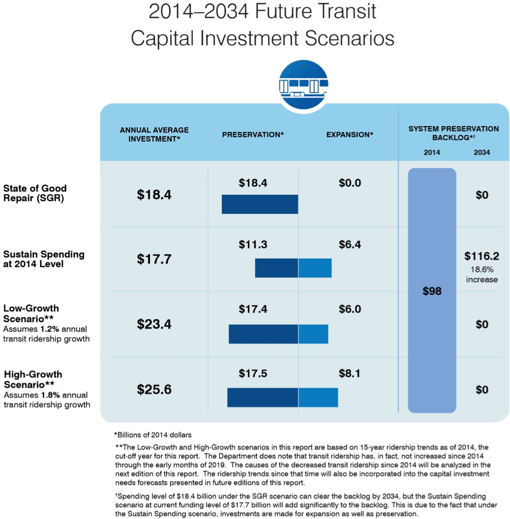
- The Sustain 2014 Spending scenario assumes that capital spending by all levels of government is sustained in constant-dollar terms at the 2014 level ($17.7 billion systemwide), including Recovery Act funds, through 2034. Assuming that the current split between expansion and preservation investments is maintained, this will allow for enough expansion to meet the national trend growth for the period 2004-2014 at 1.5 percent annual average increase, but will fall short of meeting system preservation needs. By 2034, this scenario will result in roughly $116.2 billion in deferred system preservation projects. If Recovery Act funds are not included in the baseline spending, the baseline spending would fall to $17.3 billion annually, with the deferred system preservation needs at approximately $117.2 billion.
Low-Growth Scenario
- The Low-Growth scenario assumes that transit ridership will grow at an average annual rate of 1.2 percent between 2014 and 2034. During that period, it also eliminates the current $98.0 billion system preservation backlog. The annualized cost of this scenario is $23.4 billion.
High-Growth Scenario
- The High-Growth scenario assumes that transit ridership will grow at an annual rate of 1.8 percent between 2014 and 2034. It also eliminates the current $98.0 billion system preservation backlog. The annualized cost of this scenario is $25.6 billion.