Chapter 6: Infrastructure Conditions

Pavement and bridge conditions directly affect vehicle operating costs because deteriorating pavement and bridge decks increase wear and tear on vehicles, resulting in higher repair costs. Poor pavement conditions on higher functional classification roadways, such as the Interstate System, tend to result in higher user costs related to vehicle speed. For example, a vehicle hitting a pothole at 65 miles per hour on an Interstate highway could accelerate wear and tear faster than hitting the same pothole at 25 miles per hour. Alternatively, poor pavement can increase travel time costs if poor road conditions force drivers to reduce speed.

Poor bridge conditions can lead to the imposition of weight limits, which can increase travel time costs by forcing trucks to seek alternative routes. If a bridge’s condition deteriorates to the point where it must be closed, all traffic would need to use alternative routes, potentially significantly increasing travel time costs. Highway user costs include vehicle operating costs, crash costs, and travel time costs, and are discussed in greater detail in Chapter 10.

As discussed in the Introduction to Part I, as part of the implementation of the Transportation Performance Management (TPM) framework established by the Moving Ahead for Progress in the 21st Century (MAP-21) and continued under the Fixing America's Surface Transportation (FAST) Act, a Final Rule for Pavement and Bridge Performance Measures (PM-2) was published on January 18, 2017. This rule defines pavement and bridge condition performance measures, along with minimum condition standards, target establishment, progress assessment, and reporting requirements. This edition of the C&P Report continues a gradual shift toward reporting pavement and bridge measures consistent with those specified in the PM-2 rule.

The Highway Performance Monitoring System (HPMS) is the source for all pavement-related data presented in this section. The HPMS includes information on the International Roughness Index (IRI), which is an indicator of the ride quality experienced by drivers. It also contains information on other pavement distresses, including faulting at the joints of concrete pavements, the amount of rutting on asphalt pavements, and amount of cracking on both concrete and asphalt pavements.

The National Bridge Inventory (NBI) is a record of data reported to FHWA from the States, Federal agencies, and Tribal governments on the condition of the Nation’s bridges. There are four primary data items used to determine bridge condition: deck, superstructure, substructure, and culvert condition ratings. The HPMS and NBI are discussed in greater detail later in this section (see Data Sources section).

Pavement and bridge conditions are affected both by environmental conditions and traffic volumes. Environmental conditions include factors such as freeze-thaw cycles, in which water from melted snow or ice seeps into cracks in a pavement and then freezes, causing cracks to expand, and ultimately contributing to the formation of potholes. Significant weather events such as hurricanes and tornadoes also present a risk to the Nation’s infrastructure; system resilience is discussed in further detail later in this chapter. Pavement and bridge deterioration accelerates on facilities with high traffic volumes, particularly facilities used by large numbers of heavy trucks. At certain points in the life cycle of an infrastructure asset, deterioration can happen rapidly because the impacts of traffic and the environment are cumulative. Deterioration can be mitigated through a variety of actions, including reconstruction, rehabilitation, and preventive maintenance. If corrective actions are not taken in a timely manner, deterioration of the pavement and bridges could continue until they can no longer remain in service.

Constructing new facilities or major rehabilitation is a relatively expensive undertaking. Such actions might not be economically justified until a pavement section or bridge has deteriorated to a poor condition. Such considerations are reflected in the investment scenarios presented in Part II of this report. Preventive maintenance actions are less expensive than rehabilitation and can be used to maintain and improve the quality of a pavement section or a bridge. Preventive maintenance actions, however, are less enduring than reconstruction or rehabilitation actions, and more aggressive actions would eventually need to be taken to preserve pavement and bridge quality.

Exhibit 6-1 identifies criteria for “good,” “fair,” and “poor” classifications for several individual pavement distresses, based on the information laid out in the PM-2 rule. The rule also established criteria for overall pavement ratings, based on combinations of ratings for individual distresses; for a section of pavement to be rated in good condition, its ratings for all three relevant distresses (ride quality, cracking, and rutting for asphalt pavements; ride quality, cracking, and faulting for concrete pavements) must be rated as good. For a section of pavement to be rated as poor, at least two of the relevant distresses must be rated as poor. Any pavements not rated as good or poor are classified as fair.

Exhibit 6-1: Condition Rating Classifications Used in the 23rd C&P Report

Condition Metric	Rating Criteria	Good	Fair	Poor
Pavement Ride Quality	The International Roughness Index (IRI) measures the cumulative deviation from a smooth surface in inches per mile.	IRI < 95	IRI 95 to 170	IRI > 170
Pavement Ride Quality (alternative)1	For roads functionally classified as urban minor arterials, rural or urban major collectors, or urban minor collectors, States can instead report a Present Serviceability Rating (PSR) on a scale of 0 to 5.	PSR ≥ 4.0	PSR > 2.0 and < 4.0	PSR ≤ 2.0
Pavement Cracking (Asphalt)	For asphalt pavements, cracking is measured as the percentage of the pavement surface in the wheel path in which interconnected cracks are present.	< 5%	5% to 20%	> 20%
Pavement Cracking (Jointed Plain Concrete)	For jointed plain concrete pavements cracking is measured as the percent of cracked concrete panels in the evaluated section.	< 5%	5% to 15%	> 15%
Pavement Cracking (Continuous Reinforced Concrete)	For Continuous Reinforced Concrete pavements, cracking is measured as the percent of cracking for the evaluated section.	< 5%	5% to 10%	> 10%
Pavement Rutting (Asphalt Pavements only)	Rutting is measured as the average depth in inches of any surface depression present in the vehicle wheel path.	< 0.20	0.20 to 0.40	> 0.40
Pavement Faulting (Concrete Pavements only)	Faulting is measured as the average vertical displacement in inches between adjacent jointed concrete panels.	< 0.10	0.10 to 0.15	> 0.15
Bridge Deck Condition	Ratings are on a scale from 0 “Failed” to 9 “Excellent.”	≥ 7	5 to 6	≤ 4
Bridge Superstructure Condition	Ratings are on a scale from 0 “Failed” to 9 “Excellent.”	≥ 7	5 to 6	≤ 4
Bridge Substructure Condition	Ratings are on a scale from 0 “Failed” to 9 “Excellent.”	≥ 7	5 to 6	≤ 4
Culvert Condition	Ratings are on a scale from 0 “Failed” to 9 “Excellent.”	≥ 7	5 to 6	≤ 4

¹ Under the PM-2 rule, PSR can be reported in lieu of IRI, rutting, and faulting for any component of the NHS with a posted speed limit under 40 miles per hour (e.g., border crossings, toll plazas).

Source: https://www.federalregister.gov/documents/2017/01/18/2017-00550/national-performance-management-measures-assessing-pavement-condition-for-the-national-highway

While this chapter does not include statistics for overall pavement condition ratings, it does include data on the ratings for the individual distresses for 2014. Data presented for the 2004 to 2014 period are limited to ride quality only, as data collection for the other pavement distresses began in 2010. While the PM-2 rule only requires that targets be set for the Interstate and non-Interstate components of the NHS, this chapter applies the same criteria to pavements on all Federal-aid highways. (HPMS does not collect condition data for the three-quarters of road mileage that is not on Federal-aid highways.)

The structurally deficient bridge classification criteria prior to the PM-2 rule consisted of the evaluation of six individual metrics: Deck Condition, Superstructure Condition, Substructure Condition, Culvert Condition, Structural Evaluation, and Waterway Adequacy. If one of these metrics was below the pertinent trigger value, the bridge was rated as structurally deficient. The PM-2 rule redefined the criteria for structurally deficient and made it equal to the criteria to classify bridges as in poor condition. The PM-2 rule considers only the first four of these metrics (Deck Condition, Superstructure Condition, Substructure Condition, and Culvert Condition); if any one of these criteria is rated poor, the bridge is classified as poor. A bridge is classified as good only if all of these metrics are rated as good. While the PM-2 rule only requires that targets be set for NHS bridges, this chapter applies the same criteria to all bridges.

The classification of a bridge as in poor condition or structurally deficient does not imply that the bridge is unsafe. Instead, the classification indicates the extent to which a bridge has deteriorated from its original condition when first built. A bridge with a classification of poor might experience reduced performance in the form of lane closures or load limits. If a bridge inspection determines a bridge to be unsafe, it is closed.

This section presents some pavement condition data based on actual miles of pavement and other data weighted by either lane miles or vehicle miles traveled (VMT). Some bridge data are presented based on actual bridge counts, while other data are weighted by bridge deck area or bridge traffic.

While raw counts are simplest to compute, weighting by VMT or bridge traffic gives a better sense of the extent to which poor pavement or bridge conditions are affecting the traveling public. Weighting by lane-miles or deck area aligns better with the costs that agencies would incur to improve existing pavements or bridges (i.e., it costs more to reconstruct a four-lane road than a two-lane road). The PM-2 rule requires that targets be set on a lane-mile-weighted basis for pavements and a deck area-weighted basis for bridges.

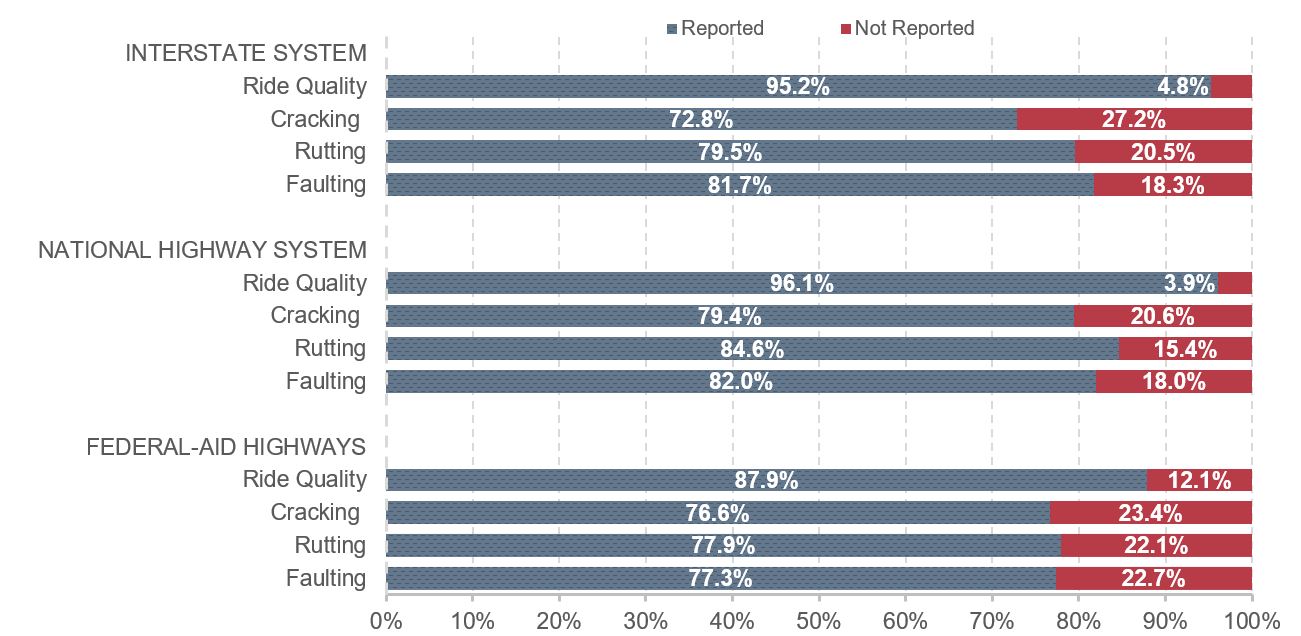
While HPMS data reporting requirements for IRI date back many years (on a universe or sample basis, depending on the type of roadway), and data reporting for cracking, rutting, and faulting date back to 2010, as of 2014, there were a number of highway sections for which these data were omitted. In some cases, States provided an alternative pavement serviceability rating (PSR) as permitted for certain types of roads; in others, no condition data were provided. Exhibit 6-2 identifies the percentage of HPMS highway segments for which data were reported in 2014 for each distress type for Interstate highways, the NHS, and Federal-aid highways.

All subsequent exhibits on pavement condition presented in this chapter are based only on those road segments for which distress data were reported. However, it should be noted that the conditions of road segments for which data were missing might not fully align with those for which data were reported, in the aggregate.

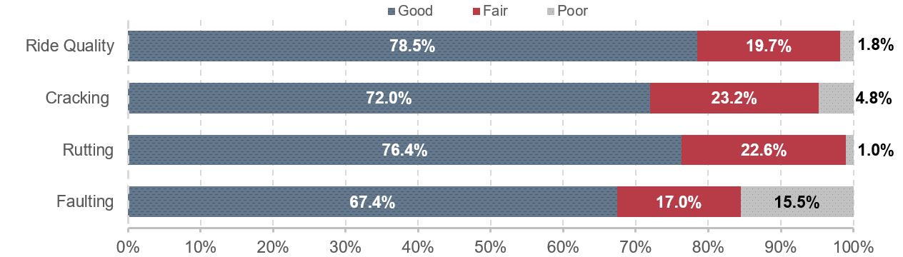
As shown in Exhibit 6-3, approximately 78.5 percent of pavements on the Interstate System (weighted by lane miles) were rated as having good ride quality (roughness) in 2014; 19.7 percent had fair ride quality, and 1.8 percent had poor ride quality. The shares of pavement rated good for cracking, rutting, and faulting were 72.0 percent, 76.4 percent and 67.4 percent, while the shares rated poor were 4.8 percent, 1.0 percent, and 15.5 percent, respectively.

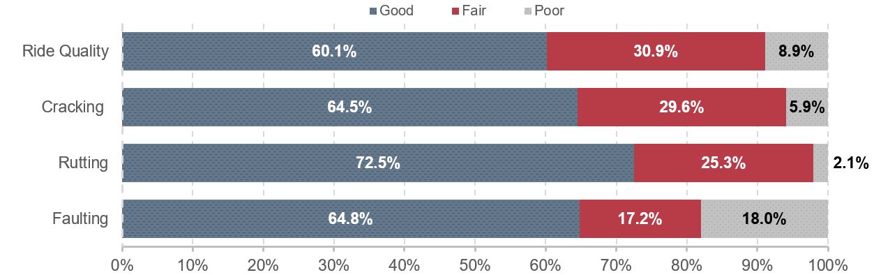
For NHS pavements, Exhibit 6-4 shows that 60.1 percent of lane miles were rated as having good ride quality in 2014; 30.9 percent had fair ride quality; and 8.9 percent had poor ride quality. Comparing the results of Exhibit 6-3 to those of Exhibit 6-4 reveals that pavement ride quality on the Interstate portion of the NHS is better than on the non-Interstate portion of the NHS.

---

Exhibit 6-2: Percentage of Pavement Data Reported

Note: Based on percentage of HPMS highway segments with data reported and not reported.

Source: Highway Performance Monitoring System.

---

Exhibit 6-3: Interstate Pavement Condition, Weighted by Lane Miles, 2014

Source: Highway Performance Monitoring System.

The lane mile-weighted shares of cracking, rutting, and faulting pavement rated good for the NHS were 64.5 percent, 72.5 percent, and 64.8 percent in 2014, all below the comparable values for Interstate highways. The share of NHS lane miles rated poor in 2014 was 5.9 percent for cracking, 2.1 percent for rutting, and 18.0 percent for faulting pavement.

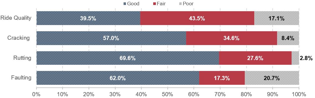
Exhibit 6-5 shows the percentage of Federal-aid highway lane miles rated good was 39.5 percent for ride quality, 57.0 percent for cracking, 69.6 percent for rutting, and 62.0 percent for faulting. All of these shares are below those reported in Exhibit 6-4 for the NHS. The percentage of Federal-aid lane miles rated poor was 17.1 percent for ride quality, 8.4 percent for cracking, 2.8 percent for rutting, and 20.7 percent for faulting; all of these values are higher than the comparable values for the NHS.

---

Exhibit 6-4: NHS Pavement Condition, Weighted by Lane Miles, 2014

Source: Highway Performance Monitoring System.

---

Exhibit 6-5: Federal-aid Highway Pavement Condition, Weighted by Lane Miles, 2014

Source: Highway Performance Monitoring System.

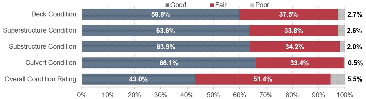
The deck-area weighted share of NHS bridges with decks in good condition is shown in Exhibit 6-6 as 59.8 percent for 2015; the shares for superstructure and substructure were 63.6 percent and 63.9 percent, respectively. The share of NHS culverts in good condition was 66.1 percent in 2015. Applying the PM-2 classification rules (all individual bridge components rated good) results in an overall share of 43.0 percent of NHS deck area rated as good.

The deck-area weighted share of NHS bridges with decks in poor condition was 2.7 percent for 2015; the shares for superstructure and substructure were 2.6 percent and 2.0 percent, respectively; the share for culverts was 0.5 percent. Applying the PM-2 classification rules (any of the individual bridge components rated poor) results in an overall share of 5.5 percent of NHS deck area rated as poor.

---

Exhibit 6-6: NHS Bridge Conditions, Weighted by Deck Area, 2015

Source: National Bridge Inventory.

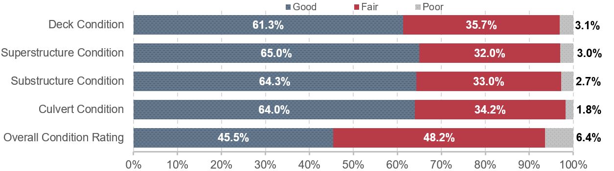
Exhibit 6-7 shows deck-area weighted condition data for all bridges. The shares of deck area rated good for deck, superstructure, and substructure were 61.3 percent, 65.0 percent, and 64.3 percent, respectively. For all culverts for which data were reported, the share rated as good was 64.0 percent in 2015. Applying the PM-2 classification rules results in an overall share of 45.5 percent of all deck area rated as good.

The deck-area weighted share of all bridges with decks in poor condition was 3.1 percent for 2015; the shares for superstructure, substructure, and culverts were 3.0 percent, 2.7 percent, and 1.8 percent, respectively. Applying the PM-2 classification rules results in an overall share of 6.4 percent of deck area rated as poor.

---

Exhibit 6-7: Systemwide Bridge Conditions, Weighted by Deck Area, 2015

Source: National Bridge Inventory.

This section presents data on changes in pavement ride quality since 2004, as well as changes in the portion of bridges rated good, fair, poor, and structurally deficient. As noted earlier, data on other pavement distresses were not collected for this full period. Pavement ride quality data are only available for Federal-aid highways.

Increases in the number of bridges and miles of roadway bridges can influence condition measures computed as shares. New roads and bridges rated in good condition can help bring up the overall average, even if the condition of existing roads and bridges remains the same or declines. However, the addition of new assets also puts strain on budgets to maintain all assets, making it more challenging to keep overall average conditions from declining.

In 1998, DOT began establishing annual targets for pavement ride quality. Since 2006, the metric reflected in DOT performance-planning documents has been the share of VMT on the NHS on pavements with good ride quality. Consequently, the pavement discussion in this section focuses on VMT-weighted measures. The bridge discussion focuses on deck-area weighted measures to be consistent with DOT performance-planning documents.

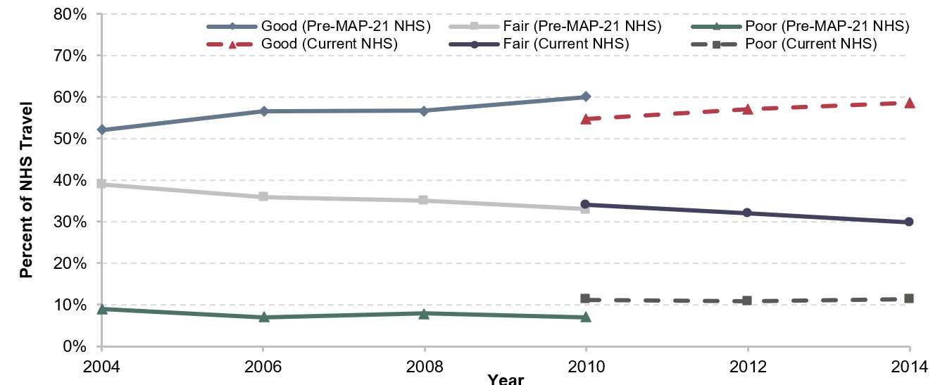
MAP-21 expanded the NHS to include most of the principal arterial mileage that was not previously included in the system. Although 2012 was the first year for which HPMS data were collected based on this expanded NHS, Exhibit 6-8 includes estimates for 2010 that were presented in the 2013 C&P Report. As reflected in a comparison of the actual 2010 values with these estimates, expanding the NHS reduced the percentage of NHS VMT on pavements with good ride quality and increased the percentage of NHS VMT on pavements with poor ride quality. On average, the additional routes added to the NHS had rougher pavements than the routes that were already part of the NHS.

The share of VMT on NHS pavements with good ride quality rose from 52 percent in 2004 to 60 percent in 2010, based on the pre-expansion NHS, and from an estimated 54.7 percent in 2010 to 58.7 percent in 2014, based on the post-expansion NHS. Combining the trends for these two separate periods translates into an average increase of more than 1 percentage point per year. From 2004 to 2010, the share of VMT on NHS pavements with poor ride quality declined from 9 percent to 7 percent; this share increased slightly from an estimated 11.2 percent to 11.4 percent from 2010 to 2014.

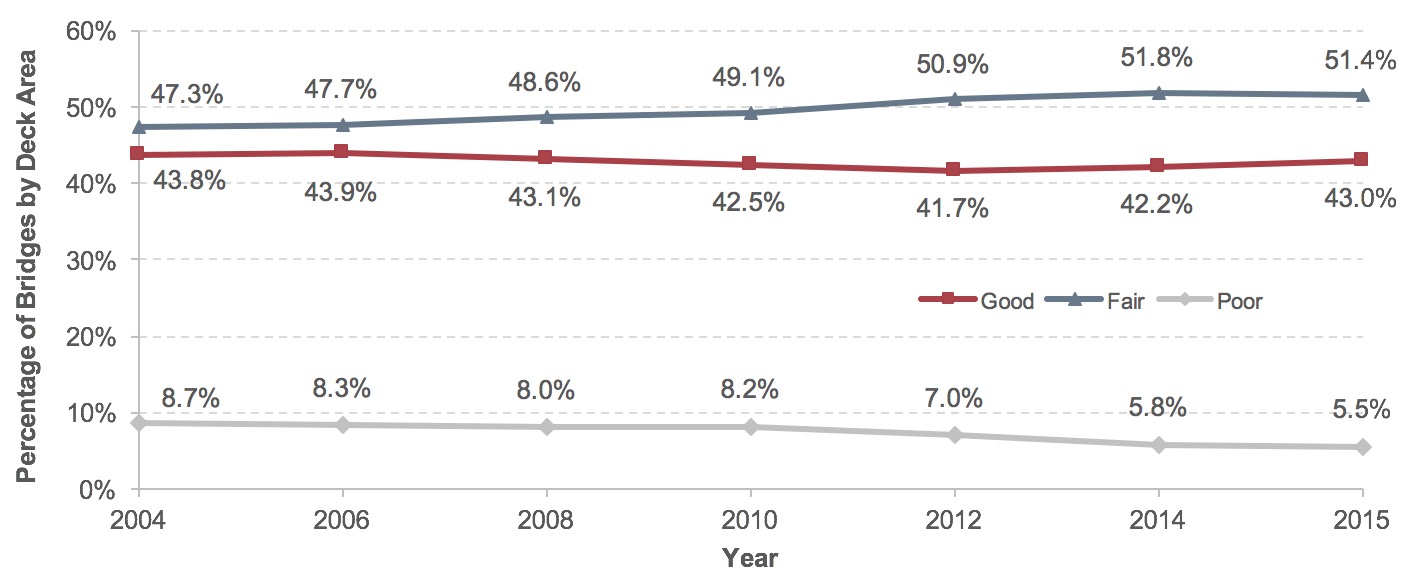
Exhibit 6-9 shows the performance of bridges on the NHS from 2004 through 2015. The share of total deck area of bridges rated poor declined from 8.7 percent in 2004 to 5.8 percent in 2014 and to 5.5 percent in 2015. The deck area of bridges in good condition also declined, from 43.8 percent in 2004 to 42.2 percent in 2014, before rebounding to 43.0 percent in 2015; the share of bridges classified as fair (i.e., not good or poor) increased over this period.

---

Exhibit 6-8: NHS Pavement Ride Quality, Weighted by VMT, 2004–2014¹

¹ Data for odd-numbered years omitted. Italicized 2010 values shown for the current NHS are estimates as presented in the 2013 C&P report. Exact values cannot be determined as the 2010 HPMS data were collected based on the pre-MAP-21 NHS. Values for the pre-MAP-21 NHS are shown as whole percentages to be consistent with how they were reported at the time in DOT performance planning documents.

Source: Highway Performance Monitoring System.

---

Exhibit 6-9: NHS Bridge Condition Ratings by Deck Area, 2004–2015¹

¹ Odd-numbered years omitted (except for 2015).

Source: National Bridge Inventory.

The expansion of the NHS under MAP-21 also increased the number of bridges; this is the major driver of the significant increase in the number of NHS bridges shown in Exhibit 6-10, from 117,485 in 2012 to 143,165 bridges in 2014. Even with the expansion, the number of structurally deficient bridges on the NHS decreased from 6,617 in 2004 to 5,951 in 2014 and to 5,479 in 2015. The number of NHS bridges in poor condition decreased from 6,395 bridges in 2004 to 5,825 bridges in 2014 and 5,358 in 2015. The total percentage of structurally deficient bridges by deck area decreased from 8.9 percent in 2004 to 6.0 percent in 2014 and to 5.6 percent in 2015.

---

Exhibit 6-10: NHS Bridges Rated Structurally Deficient or Poor, 2004–2015

	2004	2006	2008	2010	2012	2014	2015
Count
Total Bridges	115,103	115,202	116,523	116,669	117,485	143,165	143,139
Structurally Deficient Bridges	6,617	6,339	6,272	5,902	5,237	5,951	5,479
Poor Bridges	6,395	6,166	6,126	5,781	5,121	5,825	5,358
Percent Structurally Deficient
By Bridge Count	5.7%	5.5%	5.4%	5.1%	4.5%	4.2%	3.8%
Weighted by Deck Area	8.9%	8.4%	8.2%	8.3%	7.1%	6.0%	5.6%
Weighted by ADT	6.8%	6.6%	6.4%	6.0%	5.1%	4.3%	4.0%
Percent Poor
By Bridge Count	5.6%	5.4%	5.3%	5.0%	4.4%	4.1%	3.7%
Weighted by Deck Area	8.7%	8.3%	8.0%	8.2%	7.0%	5.8%	5.5%
Weighted by ADT	6.7%	6.5%	6.3%	5.9%	5.0%	4.2%	3.9%

Source: National Bridge Inventory.

Exhibit 6-11 details pavement ride quality on Federal-aid highways. The share of pavement mileage with good ride quality decreased from 43.1 percent in 2004 to 38.4 percent in 2014, but weighting the ride quality data by VMT produces significantly different results. During the same period, the share of VMT on Federal-aid highways with good ride quality increased from 44.2 percent to 47.0 percent. The implication is that pavement investment is likely being directed to parts of the system that are serving the most travelers, but that some less- traveled parts of the system are lagging behind.

Trends in terms of poor ride quality have consistently worsened based on either mileage or VMT. From 2004 to 2014 the share of miles with pavement ride quality classified as poor increased from 13.4 percent to 22.2 percent; over the same period, the share of Federal-aid highway VMT on pavements with poor ride quality increased from 15.1 percent to 17.3 percent.

---

Exhibit 6-11: Pavement Ride Quality on Federal-aid Highways, 2004–2014¹

	2004	2006	2008	2010	2012	2014
By Mileage
Good	43.1%	41.5%	40.7%	35.1%	36.4%	38.4%
Fair	43.6%	42.7%	43.5%	44.9%	43.9%	39.4%
Poor	13.4%	15.8%	15.8%	20.0%	19.7%	22.2%
Weighted by VMT
Good	44.2%	47.0%	46.4%	50.6%	44.9%	47.0%
Fair	40.7%	39.0%	39.0%	31.4%	38.4%	35.7%
Poor	15.1%	14.0%	14.6%	18.0%	16.7%	17.3%

¹ Due to changes in data reporting instructions, data for 2010 and beyond are not fully comparable to data for 2008 and prior years.

Source: Highway Performance Monitoring System.

Exhibit 6-12 shows that, based on unweighted bridge counts, the share of bridges rated as good fell from 48.2 percent in 2004 to 47.1 percent in 2014, before rising back to 47.3 percent in 2015. The comparable shares weighted by deck area and by bridge traffic were a bit lower (45.5 percent and 45.8 percent, respectively, in 2015), but showed a similar pattern across this period.

---

Exhibit 6-12: Systemwide Bridge Conditions, 2004–2015

	2004	2006	2008	2010	2012	2014	2015
Count
Total Bridges	594,100	597,561	601,506	604,493	607,380	610,749	612,845
Bridges in Good Condition	286,152	287,969	287,317	286,534	287,194	287,701	289,158
Bridges in Fair Condition	241,176	246,309	252,217	258,277	262,878	269,734	271,690
Bridges in Poor Condition	65,105	62,297	61,002	59,305	57,049	52,905	50,917
Structurally Deficient Bridges	79,971	75,422	72,883	70,431	66,749	61,365	58,791
Percent Good
By Bridge Count	48.2%	48.2%	47.8%	47.4%	47.3%	47.1%	47.3%
Weighted by Deck Area	46.1%	46.1%	45.8%	45.2%	44.7%	44.7%	45.5%
Weighted by ADT	46.4%	45.6%	44.7%	44.4%	44.0%	44.5%	45.8%
Percent Fair
By Bridge Count	40.6%	41.2%	41.9%	42.7%	43.3%	44.2%	44.4%
Weighted by Deck Area	44.3%	44.7%	45.3%	46.0%	47.3%	48.3%	48.2%
Weighted by ADT	46.1%	47.1%	48.2%	48.9%	50.2%	50.6%	49.8%
Percent Poor
By Bridge Count	12.0%	10.4%	10.1%	9.8%	9.4%	8.7%	8.3%
Weighted by Deck Area	9.4%	9.0%	8.8%	8.7%	7.8%	6.7%	6.4%
Weighted by ADT	7.3%	7.1%	7.0%	6.5%	5.7%	4.7%	4.4%
Percent Structurally Deficient
By Bridge Count	13.5%	12.6%	12.1%	11.7%	11.0%	10.0%	9.6%
Weighted by Deck Area	10.1%	9.6%	9.3%	9.1%	8.2%	7.1%	6.7%
Weighted by ADT	7.6%	7.4%	7.2%	6.7%	5.9%	4.9%	4.6%

Source: National Bridge Inventory.

The share of bridges classified as poor dropped from 11.0 percent in 2004 to 8.7 percent in 2014, dropping further to 8.3 percent in 2015. The share of bridges weighted by deck area rated poor was lower (9.4 percent in 2004, dropping to 6.7 percent in 2014 and 6.4 percent in 2015), suggesting that larger bridges are in better shape on average than smaller ones. The share of bridges weighted by average daily traffic (ADT) rated poor was even lower (7.3 percent in 2004, dropping to 4.7 percent in 2014 and 4.4 percent in 2015), suggesting that well-traveled bridges are in better shape on average than less traveled ones.

The share of bridges rated structurally deficient follows a similar pattern to those classified as poor; the numbers are uniformly higher (13.5 percent in 2004, falling to 10.0 percent in 2014 and 9.6 percent in 2015), as the structurally deficient classification also takes into account the structural evaluation and waterway adequacy appraisals from the NBI, which are not considered in the PM-2 rule definition of “poor.”

Although changes in HPMS reporting procedures in 2009 make identifying trends over the full 10-year period shown in Exhibit 6-13 and Exhibit 6-14 more challenging, it is still possible to draw some significant conclusions from the data. Rural Interstates have the best ride quality of all functional systems, with 80.7 percent of VMT on pavements with good ride quality in 2014, up from 73.7 percent in 2004. The share of urban Interstate System VMT on pavements with good ride quality from 2004 to 2014 rose sharply from 49.4 percent to 64.2 percent.

---

Exhibit 6-13: Pavement Ride Quality Rated Good, by Functional Class, Weighted by VMT, 2004–2014¹

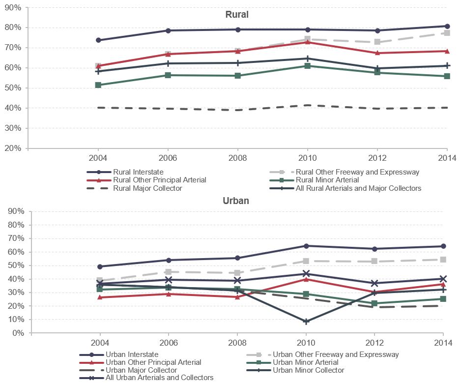
¹ Odd-numbered year data omitted. Prior to 2010, Rural Other Freeway and Expressway was included as part of Rural Other Principal Arterial; Urban Major Collector and Minor Collector were combined into a single category called Urban Collector.

Source: HPMS.

The share of rural arterial and major collector VMT on pavements with good ride quality rose from 58.3 percent in 2004 to 61.1 percent in 2014, while the comparable share of urban arterial and collector VMT rose from 35.6 percent to 40.2 percent. As noted in Chapter 1, rural areas include more miles of roadway than do urban areas, but roads in urban areas carry more VMT. Hence, rural ride quality has a greater impact on national measures of pavement condition based on mileage, whereas urban ride quality has a greater impact on national measures weighted on VMT. Higher-ordered functional systems (Interstate and other arterials) have a relatively greater impact on national measures weighted by lane miles than do lower-ordered functional systems (collectors), as these types of roadways have more lanes, on average.

In general, it can be seen in Exhibit 6-13 that roads with higher functional classifications have better ride quality than lower-ordered systems. Among the rural functional classifications, the percentage of VMT on pavements with good ride quality in 2014 ranged from 80.7 percent for rural Interstates to 40.1 percent for rural major collectors. A similar pattern is evident among most urban functional classifications, as the percentage of VMT on pavements with good ride quality in 2014 ranged from 64.2 percent for urban Interstates to 20.3 percent for urban major collectors. An exception to this general pattern was that urban minor collectors showed a higher percentage of VMT on pavements with good ride quality than did urban major collectors and urban minor arterials in 2014. It should be noted, however, that the urban minor collector category is relatively new (prior to 2010, it had been included with urban major collectors in a combined urban collector classification), and some States may not yet have adapted their data to align with the new classification structure.

Exhibit 6-14 shows share of pavements with poor ride quality by functional class. In 2014, urban major collectors had the highest percentage of VMT on poor ride quality pavements at 37.5 percent, up from 27.4 percent in 2004. Rural Interstate had the lowest VMT-weighted share of pavements with poor ride quality in 2004 at 2.2 percent, which rose to 2.6 percent by 2014. The lowest of share of VMT on poor ride quality pavements in 2014 was on “rural other freeways and expressways” at 2.4 percent; the comparable value for 2004 is unknown, as prior to 2010 these types of facilities were included in the “rural other principal arterial” category. The VMT-weighted share of VMT on all rural arterials and major collectors combined rose from 5.5 percent in 2004 to 7.4 percent in 2014; the comparable share for all urban arterials and collectors rose from 20.3 percent to 22.1 percent over this period.

Within rural areas, lower-ordered functional systems generally had higher shares of pavements with poor ride quality than did high-ordered systems. The share of VMT on rural major collector pavement with poor ride quality rose from 11.5 percent in 2004 to 15.7 percent in 2014. This pattern was generally evident in urban areas as well, with the exception of urban minor collectors, whose VMT-weighted share of poor pavement ride quality was 24.8 percent in 2014, tying that of urban other principal arterials. Among the urban functional classes, urban Interstate had the lowest share of VMT on pavements with poor ride quality, falling from 9.7 percent in 2004 to 7.2 percent in 2014.

---

Exhibit 6-14: Pavement Ride Quality Rated Poor, By Functional Class, Weighted by VMT, 2004–2014¹

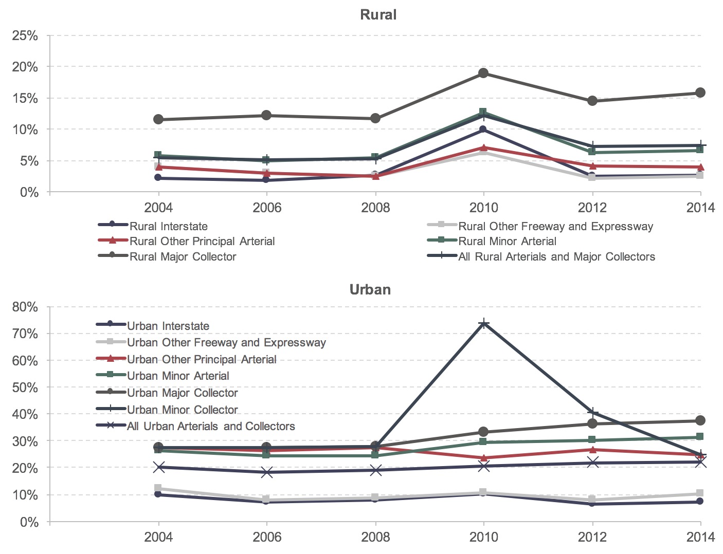
¹ Odd-numbered year data omitted. Prior to 2010, Rural Other Freeway and Expressway was included as part of Rural Other Principal Arterial; Urban Major Collector and Minor Collector were combined into a single category called Urban Collector.

Source: HPMS.

Unlike the pattern observable in Exhibit 6-13 for pavement ride quality, the classification of bridges as good does not vary relatively consistently with functional class. Exhibit 6-15 shows that the highest share of bridges in good condition was on rural other principal arterials, which declined slightly from 56.9 percent in 2004 to 56.4 percent in 2014, before dipping further to 56.1 percent in 2015. The lowest share of bridges in good condition in 2015 was 41.5 percent for rural Interstates, up slightly from 41.3 percent in 2014, but down significantly from 51.0 percent in 2004.

Among the urban functional classes, the highest share of bridges in good condition was on urban other freeways and expressways, falling from 54.3 percent in 2004 to 52.2 percent in 2014, before rising to 54.2 percent in 2015. The lowest share of urban bridges in good condition in 2015 was 42.2 percent for urban Interstates, up slightly from 41.1 percent in 2014 but down from 44.8 percent in 2004.

The overall percentages of rural and urban bridges classified as good were very similar across this period. Urban bridges had a slight advantage in 2004 (49.0 percent good for urban, versus 47.9 percent for rural), but rural bridges edged ahead by 2014 (47.2 percent good for rural versus 46.8 percent good for urban), before urban bridges reclaimed their advantage in 2015.

---

Exhibit 6-15: Bridges Rated Good, by Functional Class, 2004–2015

	2004	2006	2008	2010	2012	2014	2015
Functional Class	Percent Good Condition
Rural
Interstate	51.0%	49.3%	46.9%	44.5%	42.5%	41.3%	41.5%
Other Principal Arterial	56.9%	57.5%	56.9%	56.5%	56.5%	56.4%	56.1%
Minor Arterial	52.3%	51.7%	51.4%	50.4%	49.7%	49.7%	50.0%
Major Collector	49.3%	48.9%	48.3%	47.6%	47.8%	47.4%	47.4%
Minor Collector	46.3%	46.6%	46.1%	45.4%	45.4%	45.1%	45.0%
Local	44.9%	45.6%	45.8%	46.0%	46.2%	46.2%	46.1%
Subtotal Rural	47.9%	48.1%	47.8%	47.4%	47.4%	47.2%	47.1%
Urban
Interstate	44.8%	43.9%	42.7%	42.5%	41.1%	41.1%	42.2%
Other Freeway and Expressway	54.3%	53.6%	52.6%	52.4%	52.0%	52.2%	54.2%
Other Principal Arterial	47.2%	47.3%	46.8%	46.1%	45.9%	45.8%	46.3%
Minor Arterial	48.0%	47.4%	46.5%	46.1%	45.5%	44.9%	45.7%
Collector	49.6%	48.5%	47.3%	47.9%	48.3%	48.1%	48.3%
Local	52.0%	51.8%	51.3%	50.7%	50.8%	50.6%	50.7%
Subtotal Urban	49.0%	48.5%	47.7%	47.4%	47.0%	46.8%	47.6%
Total Good	48.2%	48.2%	47.8%	47.4%	47.3%	47.1%	47.3%

Source: National Bridge Inventory.

Exhibit 6-16 shows share of bridges classified as poor, by functional class. As was the case for pavement ride quality in Exhibit 6-14, a clear pattern is discernable with the higher functional class generally having the lowest share of bridges rated poor. The exceptions are that the share for rural other principal arterial (5.2 percent in 2004, dropping to 3.0 percent in 2014 and 2.8 percent in 2015) has fallen below that for rural Interstates (4.1 percent in 2004, dropping to 3.5 percent in 2014 and 3.2 percent in 2015), while the share for urban other freeway and expressway (5.9 percent in 2004, dropping to 3.3 percent in 2014 and 3.0 percent in 2015) has remained below that for urban Interstates (6.2 percent in 2004, dropping to 3.9 percent in 2014 and 3.7 percent in 2015).

Among all functional classes, the highest share of bridges rated in poor condition was for rural local, though this was reduced from 15.7 percent in 2004 to 13.0 percent in 2014 and 12.6 percent in 2015. The lowest share of bridges rated in poor condition was on rural other principal arterials. The share of bridges rated as poor was consistently higher in rural areas (11.7 percent in 2004, dropping to 9.5 percent in 2014 and 9.2 percent in 2015) than in urban areas (8.4 percent in 2004, dropping to 6.3 percent in 2014 and 6.0 percent in 2015).

---

Exhibit 6-16: Bridges Rated Poor, by Functional Class, 2004–2015

	2004	2006	2008	2010	2012	2014	2015
Functional System	Percent Poor Condition
Rural
Interstate	4.1%	4.2%	4.4%	4.5%	4.1%	3.5%	3.2%
Other Principal Arterial	5.2%	4.9%	4.7%	4.3%	3.7%	3.0%	2.8%
Minor Arterial	7.9%	7.8%	7.7%	7.0%	6.3%	5.7%	5.4%
Major Collector	9.8%	9.4%	9.1%	8.8%	8.5%	7.9%	7.5%
Minor Collector	11.0%	10.6%	10.5%	10.4%	9.9%	9.4%	9.2%
Local	15.7%	14.7%	14.2%	14.0%	13.8%	13.0%	12.6%
Subtotal Rural	11.7%	11.1%	10.9%	10.6%	10.2%	9.5%	9.2%
Urban
Interstate	6.2%	5.9%	5.8%	5.4%	4.7%	3.9%	3.7%
Other Freeway and Expressway	5.9%	5.7%	5.4%	4.9%	4.2%	3.3%	3.0%
Other Principal Arterial	8.9%	8.4%	8.3%	7.9%	7.4%	6.6%	5.8%
Minor Arterial	9.6%	9.4%	9.2%	8.7%	8.0%	7.4%	7.1%
Collector	10.0%	10.1%	10.0%	9.2%	8.7%	7.9%	7.4%
Local	9.8%	9.5%	9.4%	9.1%	8.7%	8.2%	8.0%
Subtotal Urban	8.4%	8.2%	8.0%	7.6%	7.0%	6.3%	6.0%
Total Poor	11.0%	10.4%	10.1%	9.8%	9.4%	8.7%	8.3%

Source: National Bridge Inventory.

Exhibit 6-17 shows pavement ride quality on Federal-aid highways by owner. As referenced in Chapter 1, State highway agencies owned 55.7 percent of Federal-aid highway mileage in 2014, while the Federal government owned 0.8 percent. The remaining 43.5 percent was owned by a combination of local governments and other State agencies.

---

Exhibit 6-17: Federal-aid Highway Pavement Ride Quality By Owner, Weighted by Lane Miles, 2014

	Federal	State Highway Agencies	Other
Federal-aid Highways1
Good	63.2%	62.9%	27.7%
Fair	28.0%	29.9%	34.7%
Poor	8.8%	7.2%	37.5%

¹ Based on IRI data only, rather than a combination of IRI and PSR data.

Source: HPMS.

Weighted by lane miles, approximately 63.2 percent of federally owned routes on Federal-aid highways were classified as having good ride quality in 2014; the comparable share for State-owned Federal-aid highways was 62.9 percent. The share of Federal-aid lane miles owned by other entities with good ride quality was much lower, at 27.7 percent. Only 7.2 percent of State-owned Federal-aid highway lane miles had poor ride quality in 2014; the comparable shares for Federal and Other were 8.8 percent and 37.5 percent, respectively.

Differences in condition by owner are less dramatic for bridges than for pavements. As shown in Exhibit 6-18, bridges owned by local governments had a higher share rated good (47.9 percent) than State-owned (46.7 percent) or federally owned (47.7 percent) bridges. However, local governments also had a higher share of bridges rated poor (10.8 percent) than at the State (5.8 percent poor) or Federal (7.2 percent poor) levels. The 0.2 percent of bridges that are owned by private entities or for which ownership was not identified in the NBI have considerably lower shares rated good (32.4 percent) and higher shares rated poor (24.8 percent) than bridges owned by Federal, State, or local governments.

---

Exhibit 6-18: Bridge Conditions, by Owner, 2015¹

	Federal	State	Local	Private/Other2	Total
Percentages
Percent Owned	1.7%	48.3%	49.8%	0.2%	100.0%
Classified as Good	47.7%	46.7%	47.9%	32.4%	47.3%
Classified as Fair	44.9%	47.6%	41.3%	42.4%	44.4%
Classified as Poor	7.2%	5.8%	10.8%	24.8%	8.3%

¹ These data only reflect bridges for which inspection data were submitted to the NBI.

² The National Bridge Inspection Standards apply to all structures defined as highway bridges located on all public roads. Privately-owned bridges are not required to be inspected nor data submitted to FHWA. Inspection data on some privately-owned bridges are provided voluntarily, but there is an unknown number of privately-owned highway bridges for which data are not provided to the NBI.

Source: National Bridge Inventory.

Exhibit 6-19 identifies the age composition of all highway bridges in the Nation. As of 2015, approximately 34.7 percent of the Nation’s bridges were between 26 and 50 years old. For NHS bridges, 41.1 percent were in this age range, while 52.1 percent of the Interstate bridges fell into this age range. Approximately 35.9 percent of all bridges are 51 years old or older. The percentages of NHS and Interstate bridges in this group are 33.0 percent and 31.5 percent, respectively.

Exhibit 6-20 identifies the distribution of poor condition bridges within the age ranges presented in Exhibit 6-19. The percentage of bridges classified as poor generally tends to rise as bridges age. Although only 6.2 percent of bridges in the 26-to-50-year age group are rated as poor, the percentage is 12.8 percent for bridges 51 to 75 years of age and 21.3 percent for bridges 76 to 100 years of age. Similar patterns are evident in the data for NHS and Interstate System bridges, although the overall percentage of poor bridges for these systems is lower than for the national bridge population.

The age of a bridge structure is just one indicator of its serviceability, or condition under which a bridge is still considered useful. A combination of several factors influences the serviceability of a structure, including the original design; the frequency, timeliness, effectiveness, and appropriateness of the maintenance activities implemented over the life of the structure; the loading to which the structure has been subjected during its life; the climate of the area where the structure is located; and any additional stresses from events such as flooding to which the structure has been subjected. As an example, two structures built at the same time using the same design standards and in the same climate can have very different serviceability levels. The first structure might have had increased heavy truck traffic, lack of preventive maintenance of the deck or the substructure, or lack of rehabilitation work. The second structure could have had the same increases in heavy truck traffic but received timely preventive maintenance activities on all parts of the structure and proper rehabilitation activities. In this example, the first structure would have a low serviceability level, while the second structure would have a high serviceability level.

---

Exhibit 6-19: Bridges by Age, 2015

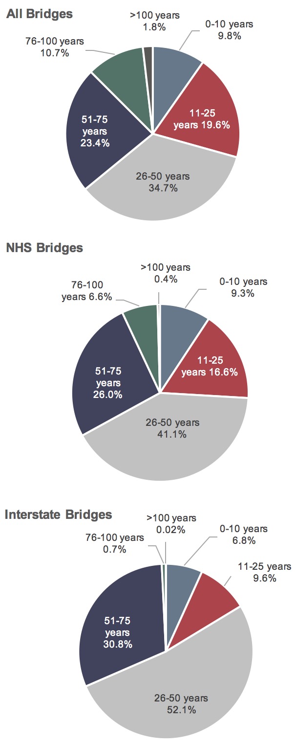
Source: National Bridge Inventory.

---

Exhibit 6-20: Bridges Rated Poor, by Age, 2015

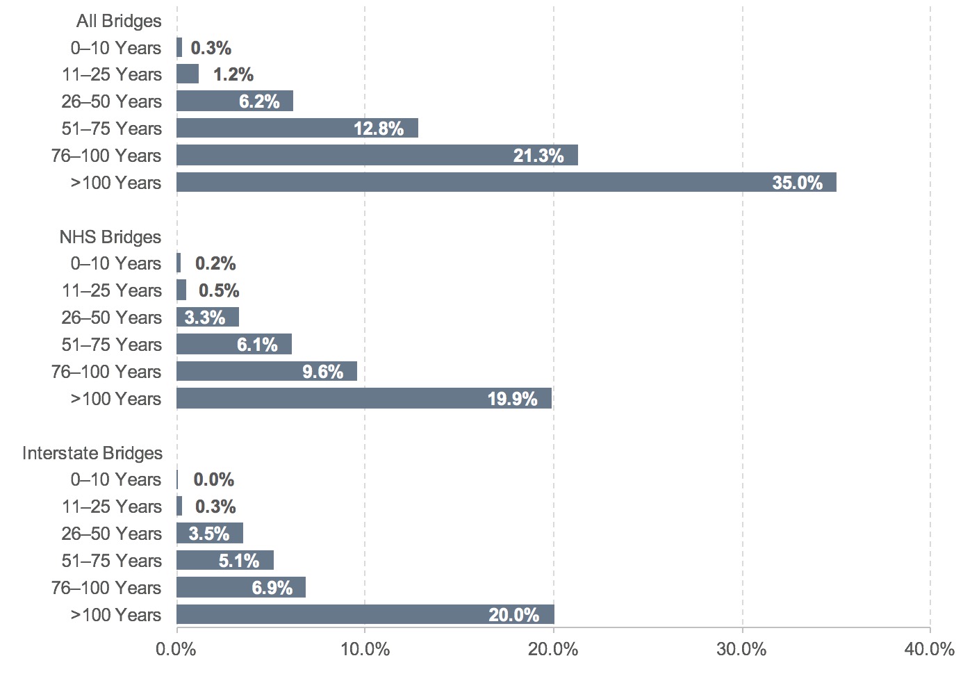
Source: National Bridge Inventory.

Transportation agencies have limited resources—both staff and budgets—when constructing or repairing roads and bridges. This constraint creates the need to work more efficiently and focus on technologies and processes that produce the best results.

Improving project delivery is a high priority for FHWA. Projects that are delivered faster and more efficiently can minimize the disruption to stakeholders that construction causes. Through its Every Day Counts initiative, FHWA is partnering with State departments of transportation and stakeholders to identify and rapidly deploy proven but underutilized innovations to shorten the project delivery process, enhance roadway safety, reduce congestion, and improve environmental sustainability.

The concept is to select projects that improve existing highways and bridges with emphasis on minimizing life-cycle costs. Applying a preservation treatment at the right time (when), on the right project (where), with quality materials and construction (how) is a critical investment strategy for optimizing infrastructure performance.

In addition to preservation actions, new construction techniques—such as ultra-high performance concrete connections for prefabricated bridge elements—can speed construction of a new bridge and result in a higher quality of construction. Planning techniques, such as the Transportation Asset Management Plan (TAMP), can aid in the strategic management of the activities to be undertaken to reach and maintain a state of good repair for all transportation facilities.

Highway pavements and bridges are subject to traffic loads and environmental elements that will contribute to their deterioration over time. Preventive maintenance treatments are a tool that can slow this decline. When the right treatment is applied at the right time with quality materials and construction, these practices offer a proven, cost-effective approach to extending the overall service life of pavements and bridges with fewer costly repairs.

Preventive maintenance includes work that is planned and performed to improve or sustain the condition of the transportation facility in a state of good repair. Preventive maintenance activities generally do not add capacity or structural value but do restore or maintain the transportation facility’s overall condition.

Benefits of the application of proper and timely application of preservation actions include:

• Economy. Whole-life planning for pavements and bridges defines expectations and risks for the long term and provides more stability to the cost of operating and maintaining pavements and bridges.
• Performance. Identifying preventive maintenance policies and strategies at the network level provides a cost-effective alternative for extending the performance period for pavements and bridges and reducing the need for frequent or unplanned reconstruction.
• Sustainability. A well-defined project strategy that includes preventive maintenance will aid in setting achievable performance targets.
• Flexibility. Retaining a mix of successful treatments in the preventive maintenance toolbox provides agencies greater flexibility in placing the right treatment on the right pavement or bridge at the right time.
• Savings. Improved performance and fewer failures keep a pavement and bridge network in a state of good repair at a lower cost.

In contrast, capital improvement projects involve work to improve the structural condition of the pavement or bridge. The benefit of this approach is a return of the pavement or bridge to a state of good repair through reconstruction or a major improvement through major rehabilitation work. Capital improvement is usually undertaken when a pavement or bridge cannot continue to meet the needs of the transportation network due to excessive deterioration or due to a lack of capacity. It is a more costly and time-consuming alternative than preservation.

Pavement preventive maintenance is one of the strategies to maintain roadways in a state of good repair. Pavements deteriorate as a result of many different forces, but the predominant factors affecting pavement performance are the vehicle loads and environmental elements to which pavements are exposed over their lifetime. Today, most highway agencies accept that an effective pavement preventive maintenance program will slow the rate of pavement deterioration while also providing a safer, smoother ride to the traveling public. Pavement preventive maintenance programs based on the 3Rs—right treatment, right pavement, and right time—have been proven to extend pavement life while saving money.

The program Every Day Counts-4 is promoting quality construction and materials practices that apply to both flexible and rigid pavements. For flexible pavements, these include using improved specifications for thin asphalt surfacings, such as chip seals, scrub seals, slurry seals, microsurfacing, and ultrathin bonded wearing courses; following improved construction practices; and using the right equipment to place these treatments. Rigid pavement strategies include the rapid retrofitting of dowel bars to reduce future faulting; the use of new, fast-setting partial- and full-depth patching materials to create a long-lasting surface; advanced pavement removal techniques to accelerate patching construction times; and advancements in diamond grinding that contribute to smoother and quieter pavement surfaces with enhanced friction.

Pavement condition data are reported to FHWA through the HPMS. The HPMS requires reporting for Federal-aid highways only, which represent about a quarter of the Nation’s road mileage but carry approximately five-sixths of the Nation’s travel. States are not required to report detailed data on roads functionally classified as rural minor collectors, rural local, or urban local, which make up the remaining three-quarters of the Nation’s road mileage.

PMS contains data on multiple types of pavement distresses. Data on pavement roughness are used to assess the quality of the ride that highway users experience. For some functional systems, States can report a general Pavement Serviceability Rating value in place of an actual measurement of pavement roughness through the IRI. Other measures of pavement distress include pavement cracking, pavement rutting (surface depressions in the vehicle wheel path, generally relevant only to asphalt pavements), and pavement faulting (the vertical displacement between adjacent jointed sections on concrete pavements).

Bridge condition data are reported to FHWA through the NBI, which reflects information gathered by States, Federal agencies, and Tribal governments during their safety inspections of bridges. Most inspections occur once every 24 months. If a structure shows advanced deterioration, the frequency of inspections might increase so that the structure can be monitored more closely. Based on certain criteria, structures that are in satisfactory or better condition may be inspected between 24 and 48 months with prior FHWA approval. Approximately 83 percent of bridges are inspected every 24 months, 12 percent every 12 months, and 5 percent on a maximum 48-month cycle.

Bridge inspectors are trained to inspect bridges based on, as a minimum, the criteria in the National Bridge Inspection Standards. Inspections are required for all 611,845 bridges and culverts with spans of more than 20 feet located on public roads.

The NBI database contains condition classifications on the three primary components of a bridge: deck, superstructure, and substructure. The bridge deck is the surface on which vehicles travel and is supported by the superstructure. The superstructure transfers the load of the deck and bridge traffic to the substructure, which provides support for the entire bridge. Such classifications are not reported for the 135,810 culverts represented in the NBI, as culverts are self-contained units typically located under roadway fill, and thus do not have a deck, superstructure, or substructure. As a result, they are assigned a separate culvert rating.

Weather events present significant risks to the safety, reliability, and sustainability of the Nation’s transportation infrastructure and operations and can affect the life cycle of transportation systems. Storm surges can inundate coastal roads, necessitate more emergency evacuations, and require costly (and sometimes recurring) repairs to damaged infrastructure. Inland flooding can disrupt traffic, damage culverts, and reduce service life. High heat can degrade materials, resulting in shorter replacement cycles and higher maintenance costs.

Given the long life span of transportation assets, planning for system preservation and safe operation under current and future conditions constitutes responsible risk management. The FAST Act expands the scope of the metropolitan planning process to “improve the resiliency and reliability of the transportation system.” It also requires that metropolitan transportation plans contain strategies that “reduce the vulnerability of the existing transportation infrastructure to natural disasters.”

For the statewide transportation planning process, the FAST Act expands the scope of consideration to include projects, strategies, and services that will improve the resilience and reliability of the transportation system. The Moving Ahead for Progress in the 21st Century Act (MAP-21) requires States to develop risk-based asset management plans for the National Highway System. On October 24, 2016, FHWA published a notice of final rulemaking in the Federal Register describing the process for developing these State risk-based asset management plans.

This section reports on the quantity, age, and physical condition of transit assets, which are factors that determine how well the infrastructure can support an agency’s objectives and set a foundation for consistent measurement. Transit assets include vehicles, stations, guideway elements, track, rail yards, administrative facilities, maintenance facilities, maintenance equipment, power systems, signaling systems, communication systems, and structures that carry elevated or subterranean guideways. Chapter 4 addresses issues relating to the operational performance of transit systems.

FTA uses a numerical rating scale ranging from 1 to 5, detailed in Exhibit 6-21, to describe the relative condition of transit assets. A rating of 4.8 to 5.0, or “excellent,” indicates that the asset is in nearly new condition or lacks visible defects. The midpoint of the “marginal” rating (2.5) is the threshold below which the assets are considered not in a state of good repair (SGR). At the other end of the scale, a rating of 1.0 to 1.9, or “poor,” indicates that the asset needs immediate repair and does not support satisfactory transit service.

FTA uses the Transit Economic Requirements Model (TERM) to estimate the condition of transit assets for this report. This model consists of a database of transit assets and deterioration schedules that express asset conditions principally as a function of an asset’s age. Vehicle condition is based on the vehicle’s maintenance history and an estimate of the major rehabilitation expenditures, in addition to vehicle age. The conditions of wayside control systems and track are based on an estimate of use (revenue miles per mile of track) in addition to age. For the purposes of this report, SGR is defined using TERM’s numerical condition rating scale. Specifically, this report considers an asset to be in SGR when the physical condition of that asset is at or above a condition rating value of 2.5 (the midpoint of the marginal range). An entire transit system would be in SGR if all of its assets have an estimated condition value of 2.5 or higher. The SGR benchmark presented in Chapter 8 represents the level of investment required to attain and maintain this definition of SGR by rehabilitating or replacing all assets having estimated condition ratings that are less than this minimum condition value.

---

Exhibit 6-21: Definitions of Transit Asset Conditions

Rating	Condition	Description
Excellent	4.8–5.0	No visible defects, near-new condition.
Good	4.0–4.7	Some slightly defective or deteriorated components.
Adequate	3.0–3.9	Moderately defective or deteriorated components.
Marginal	2.0–2.9	Defective or deteriorated components in need of replacement.
Poor	1.0–1.9	Seriously damaged components in need of immediate repair.

Source: Transit Economic Requirements Model.

In 2012, the Moving Ahead for Progress in the 21st Century Act (MAP-21) directed FTA to develop a transit asset management (TAM) rule to establish a strategic and systematic process of operating, maintaining, and improving public transportation capital assets effectively through their entire life cycle. TAM is a business model that prioritizes funding based on the condition of transit assets, to achieve or maintain transit networks in SGR.

FTA has estimated typical deterioration schedules for vehicles, maintenance facilities, stations, train control systems, electric power systems, and communication systems through special on-site engineering surveys. Transit vehicle conditions also reflect the most recent information on vehicle age, use, and level of maintenance from the National Transit Database (NTD); the information used in this edition of the C&P Report is from 2014. Age information for all other assets is collected through special surveys. Average maintenance expenditures and major rehabilitation expenditures for vehicles are also available on a modal basis. When calculating conditions, FTA assumes that agency maintenance and rehabilitation expenditures for a particular mode are the same average value for all vehicles the agency operates in that mode. Because agency maintenance expenditures can fluctuate from year to year, TERM uses a 5-year average.

The deterioration schedules applied for track and guideway structures are based on special studies. Appendix C presents a discussion on the methods used to calculate deterioration schedules and the sources of data on which deterioration schedules are based.

Condition estimates in each edition of the C&P Report are based on up-to-date asset inventory information that reflects updates in TERM’s asset inventory data. Annual data from NTD were used to update asset records for the Nation’s transit vehicle fleets. In addition, updated asset inventory data were collected from 30 of the Nation’s largest rail and fixed-route bus transit agencies to support analysis of nonvehicle needs. Because these data are not collected annually, it is not possible to provide accurate time-series analysis of nonvehicle assets. FTA is working to develop improved data in this area. Appendix C provides a more detailed discussion of TERM’s data sources. Exhibit 6-22 shows the distribution of asset conditions, by replacement value, across major asset categories for the entire U.S. transit industry.

Condition estimates for assets are weighted by the replacement value of each asset. This weighting accounts for the fact that assets vary substantially in replacement value. For example, a $1 million railcar in poor condition is a much bigger problem than a $1,000 turnstile in similar condition. To illustrate the calculation involved, the cost-weighted average of a $100 asset in condition 2.0 and a $50 asset in condition 4.0 would be (100×2.0+50×4.0)/(100+50)=2.67. The unweighted average would be (2+4)/2=3.

---

Exhibit 6-22: Distribution of Asset Physical Conditions by Asset Type for All Modes

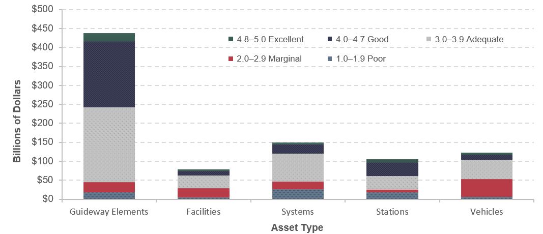
Note: Includes both replaceable assets, which should be replaced once they are below condition 2.5, and nonreplaceable assets, which should be rehabilitated once they are below condition 2.5.

Source: Transit Economic Requirements Model (TERM) and National Transit Database.

The total value of the transit infrastructure in the United States for 2014 was estimated at $894.2 billion (in 2014 dollars). These estimates, presented in Exhibit 6-23, are based on asset inventory information in TERM. They exclude the value of assets belonging to special service operators that do not report to NTD. Rail assets totaled $786.4 billion, or roughly 86 percent of all transit assets. Nonrail assets were estimated at $107.8 billion. Joint assets totaled $14.7 billion; these are assets that serve more than one mode within a single agency and can include administrative facilities, intermodal transfer centers, agency communications systems (e.g., telephone, radios, and computer networks), and vehicles used by agency management (e.g., vans and automobiles).

Note that U.S. transit asset holdings can be further broken out into replaceable vs nonreplaceable assets, with the two types of assets accounting for roughly 62 percent and 38 percent of all transit assets by value, respectively. Replaceable assets have an expected useful service life, after which the asset will require replacement. Many types of replaceable assets also require one or more rehabilitations throughout their life to ensure their full service life is attained. In contrast, nonreplaceable assets, such as subway tunnels and historic rail cars, are expected to remain in service indefinitely and hence have no planned date of retirement. For needs-assessment purposes, these assets are treated as having an infinite service life. However, all nonreplaceable assets do require periodic—in some cases annual—rehabilitation investments to maintain them in SGR. Estimates of deferred maintenance and deferred rehabilitation of nonreplaceable assets are counted toward the SGR backlog.

---

Exhibit 6-23: Estimated Value of the Nation's Transit Assets, 2014

	Value (in Billions of 2014 Dollars)
Transit Asset	Nonrail	Rail	Joint Assets	Total
Replaceable Assets
Maintenance Facilities	$39.0	$31.3	$8.2	$78.4
Guideway Elements	$3.8	$147.7	$0.0	$151.5
Stations	$4.3	$50.3	$0.8	$55.4
Systems	$5.1	$141.0	$3.9	$150.0
Vehicles	$51.7	$68.9	$1.3	$121.9
Total: Replaceable Assets	$103.8	$439.2	$14.2	$557.2
Non-Replaceable Assets
Guideway Elements	$3.5	$282.9	$0.5	$286.9
Stations	$0.0	$49.4	$0.0	$49.4
Vehicles	$0.4	$0.2	$0.0	$0.6
Total: Non-Replaceable Assets	$3.9	$332.6	$0.5	$337.0
Total: All Assets	$107.7	$771.8	$14.7	$894.2

Note: The value of the asset is based on an estimated replacement value, including for assets that are estimated to be nonreplaceable.

Source: Transit Economic Requirements Model (TERM).

Bus vehicle age and condition are reported by vehicle type for 2004 to 2014 in Exhibit 6-24. Fleet count figures since 2008 reflect the number of transit buses in both urban and rural areas. When measured across all vehicle types, the average age of the Nation’s bus fleet remained essentially unchanged, at approximately 6 years, from 2004 through 2014. Similarly, the average condition rating for all bus types (calculated as the weighted average of bus asset conditions, weighted by asset replacement value) stayed relatively constant, remaining near the bottom of the adequate range over the 10-year period. The percentage of vehicles below the SGR replacement threshold (condition level 2.5) was about 15 percent over this same period. Although this observation holds true across all vehicle types, the percentage of full-size buses (the vehicle type that supports most fixed-route bus services) below the SGR replacement threshold increased from 10.4 percent in 2012 to 16.0 percent in 2014.

The Nation’s transit road vehicle fleet has grown at an average annual rate of roughly 3 percent since 2004, with most of this growth concentrated in two vehicle types: cutaways and vans. The large increase in the number of vans reflects both the needs of an aging population (paratransit services) and an increase in the popularity of vanpool services. In contrast, the number of full- and medium-sized buses has remained relatively flat since 2004.

Exhibit 6-25 presents the age distribution of the Nation’s transit buses, and Exhibit 6-26 presents the age distribution of the Nation’s transit vans, minivans, and autos. Note that full-size buses and vans account for the highest proportion (roughly 49 percent) of the Nation’s rubber-tire transit vehicles. Although most vans are retired by age 8 and most buses by age 15, roughly 5 to 20 percent of these fleets remain in service well after their typical retirement ages.

---

Exhibit 6-24: Transit Bus Fleet Count, Age, and Condition, 2004–2014

	2004	2006	2008	2010	2012	2014
Articulated Buses
Fleet count	3,363	3,422	3,900	4,654	4,836	5,373
Average Age (Years)	5.3	5.4	6.3	6.6	7.0	7.2
Average Condition Rating	3.5	3.3	3.2	3.2	3.2	3.2
Below Condition 2.5 (Percent)	6.6%	2.5%	1.4%	2.9%	1.7%	13.8%
Full-Size Buses
Fleet count	45,539	44,866	45,999	45,783	45,314	45,717
Average Age (Years)	7.3	7.4	7.9	7.8	8.0	8.4
Average Condition Rating	3.2	3.1	3.1	3.1	3.1	3.0
Below Condition 2.5 (Percent)	14.5%	11.0%	11.6%	11.0%	10.4%	16.0%
Mid-Size Buses
Fleet count	7,080	6,875	7,577	8,169	7,615	7,753
Average Age (Years)	8.1	8.1	8.2	7.9	7.3	7.6
Average Condition Rating	3.1	3.0	3.0	3.1	3.2	3.1
Below Condition 2.5 (Percent)	17.7%	17.0%	14.4%	14.3%	11.2%	10.3%
Small Buses
Fleet count	6,868	7,539	8,689	8,743	8,434	8,267
Average Age (Years)	5.5	6.1	6.5	6.7	6.7	7.1
Average Condition Rating	3.3	3.2	3.1	3.1	3.1	3.0
Below Condition 2.5 (Percent)	12.0%	11.4%	15.8%	18.4%	19.6%	22.7%
Cutaways
Fleet count	8,481	9,427	19,477	23,268	26,983	26,753
Average Age (Years)	4.2	4.3	4.6	4.1	4.4	4.8
Average Condition Rating	3.5	3.5	3.4	3.6	3.4	3.3
Below Condition 2.5 (Percent)	13.7%	13.0%	18.6%	16.4%	15.4%	16.7%
Subtotal: Bus
Total Fleet count	71,331	72,129	85,642	90,617	93,182	93,863
Weighted Average Age (Years)	6.7	6.8	7.0	6.7	6.7	7.1
Weighted Average Condition Rating	3.2	3.2	3.2	3.2	3.2	3.1
Below Condition 2.5 (Percent)	14.1%	11.5%	13.4%	13.0%	12.3%	16.2%
Vans
Fleet count	17,698	20,714	28,846	30,650	28,759	29,207
Average Age (Years)	3.4	3.2	3.7	3.6	3.8	3.8
Average Condition Rating	3.4	3.5	3.4	3.4	3.3	3.3
Below Condition 2.5 (Percent)	18.9%	19.1%	25.3%	20.0%	25.7%	27.2%
Total: Bus and Van
Total Fleet count	89,029	92,843	114,488	121,267	121,941	123,070
Weighted Average Age (Years)	6.1	6.0	6.1	5.9	6.0	6.3
Weighted Average Condition Rating	3.4	3.5	3.4	3.4	3.3	3.3
Below Condition 2.5 (Percent)	18.9%	19.1%	25.3%	20.0%	25.7%	27.2%

Note: Table excludes NTD records with no Date Built values.

Note: Rural fleet not included in period 2004–2007 due to lack of data.

Sources: Transit Economic Requirements Model (TERM); National Transit Database.

---

Exhibit 6-25: Age Distribution of Fixed-Route Buses, 2014

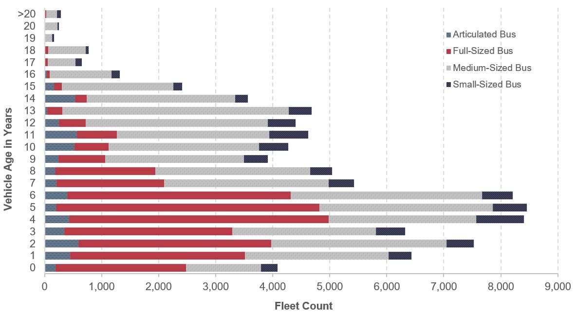
Source: Transit Economic Requirements Model (TERM) and National Transit Database.

---

Exhibit 6-26: Age Distribution of Vans, Minivans, Autos, and Cutaways, 2014

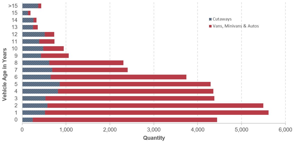
Source: Transit Economic Requirements Model (TERM) and National Transit Database.

Note that the share of the bus fleet with an average age below their expected average useful life (Exhibit 6-25) was quite high in 2014. Most of the buses in the national fleet were 8 years old or less.

The more comprehensive capital asset data described above enable reporting of a more complete picture of the overall condition of bus-related assets. Exhibit 6-27 shows TERM estimates of current conditions for the major categories of fixed-route bus assets. Vehicles comprise roughly half of all fixed-route bus assets, and maintenance facilities make up roughly one-third. Roughly one-third of bus maintenance facilities are rated below condition 3.0, compared to roughly one-half for bus, paratransit, and vanpool vehicles.

---

Exhibit 6-27: Distribution of Estimated Asset Conditions by Asset Type for Fixed-Route Bus

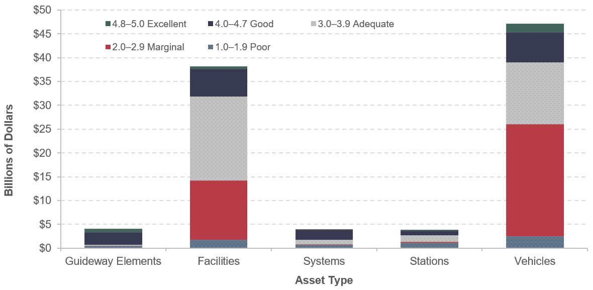
Source: Transit Economic Requirements Model (TERM).

NTD compiles annual data on all rail vehicles; these data are shown in Exhibit 6-28, broken down by major category. Measured across all rail vehicle types, the average age of the Nation’s rail fleet has remained essentially unchanged, between 19 and 20 years old, since 2004. The average condition of all rail vehicle types (calculated as the weighted average of vehicle conditions, weighted by vehicle replacement cost) is also relatively unchanged, remaining near 3.5 since 2004. The percentage of vehicles below the SGR replacement threshold (condition 2.5) has remained between 2.8 and 4.2 percent since 2004. Note that, although this observation holds across all vehicle types, the analysis suggests that most vehicles in lesser condition occur in the light and heavy rail fleets. Moreover, most light rail vehicles with an estimated condition of less than 2.5 are historic streetcars and trolley cars with an average age of 75 years. Given their historic vehicle status, the estimated condition of these vehicles (determined primarily by age) should be viewed as a rough approximation, relative to all other reported rail vehicles.

---

Exhibit 6-28: Rail Fleet Count, Age, and Condition, 2004–2014

	2004	2006	2008	2010	2012	2014
Commuter Rail Locomotives
Fleet count	710	740	790	822	877	898
Average Age (Years)	17.8	16.7	19.6	19.4	17.8	19.5
Average Condition Rating	3.7	4.0	3.6	3.6	3.7	3.7
Below Condition 2.50 (Percent)	0.0%	0.0%	0.0%	0.0%	1.8%	1.8%
Commuter Rail Passenger Coaches
Fleet count	3,513	3,671	3,539	3,711	3,758	3,742
Average Age (Years)	17.7	16.8	19.9	19.1	20.2	18.9
Average Condition Rating	3.8	4.1	3.6	3.7	3.6	3.6
Below Condition 2.50 (Percent)	0.0%	0.0%	0.0%	0.0%	0.4%	4.7%
Commuter Rail Self-Propelled Passenger Coaches
Fleet count	2,470	2,933	2,665	2,659	2,930	2,945
Average Age (Years)	23.6	14.7	18.9	19.7	19.7	17.5
Average Condition Rating	3.7	3.8	3.7	3.7	3.6	3.7
Below Condition 2.50 (Percent)	0.0%	0.0%	0.0%	0.0%	0.0%	0.1%
Heavy Rail
Fleet count	11,046	11,075	11,570	11,648	11,587	11,859
Average Age (Years)	19.8	22.3	21.0	18.8	19.9	20.7
Average Condition Rating	3.4	3.3	3.3	3.4	3.4	3.4
Below Condition 2.50 (Percent)	5.6%	5.5%	6.1%	5.2%	3.7%	11.4%
Light Rail1
Fleet count	1,884	1,832	2,151	2,222	2,241	2,416
Average Age (Years)	16.5	14.6	17.1	18.1	14.6	17.8
Average Condition Rating	3.6	3.7	3.6	3.5	3.6	3.5
Below Condition 2.5 (Percent)	9.3%	6.4%	7.1%	6.9%	6.3%	2.8%
Total Rail
Total Fleet count	19,623	20,251	20,715	21,062	21,393	21,860
Weighted Average Age (Years)	19.5	19.3	20.1	18.9	19.3	19.6
Weighted Average Condition Rating	3.5	3.6	3.5	3.5	3.5	3.5
Below Condition 2.5 (Percent)	4.1%	3.6%	4.2%	3.6%	2.8%	3.1%

¹Excludes vintage streetcars.

Source: Transit Economic Requirements Model and National Transit Database.

From 2004 to 2014, the Nation’s rail transit fleet grew at an average annual rate of roughly 1.8 percent. This rate of growth was due largely to the rate of increase in the heavy rail fleet (which represents slightly more than half the total fleet and grew at an average annual rate of 1.4 percent over this period). In contrast, the annual rate of increase in commuter rail locomotive and commuter rail self-propelled passenger coach fleets has been appreciably higher, averaging approximately 3.4 percent and 3.1 percent, respectively, while accounting for only 4 and 13 percent of the total fleet count during the 10-year period. The higher growth rates for these rail transit types may again reflect recent rail transit investments in small and medium-sized urban areas where the size and population density do not justify the greater investment needed for heavy rail construction.

Exhibit 6-29 presents the age distribution of the Nation’s heavy rail, light rail, and commuter rail transit vehicles. Heavy rail vehicles account for more than half the Nation’s rail fleet, whereas light rail, a mode more frequently found in smaller rail markets, accounts for only 11 percent of rail vehicles. Roughly one-third of heavy rail and commuter rail vehicles are more than 25 years old—with close to 3,000 heavy and commuter rail vehicles exceeding 35 years in age. Just under half (49 percent) of all rail vehicles, including 51 percent of commuter rail vehicles and 57 percent of heavy rail vehicles, are located in the greater New York City area (which includes portions of New Jersey and Connecticut), the Nation’s largest transit market.

Comparing the results in Exhibit 6-29 with the age distribution of transit buses and vans in Exhibit 6-25 and Exhibit 6-26, rail vehicles lack the relatively clear pattern of preferred retirement age that is found in buses and vans. Exhibit 6-30 presents the age distribution of the Nation’s hybrid rail, streetcar, and other rail transit vehicles. Streetcar rail vehicles account for nearly two-thirds of the vehicles presented in Exhibit 6-30, while hybrid rail vehicles account for 13 percent. Roughly three-fourths of streetcar rail vehicles are more than 25 years old, with about one-fourth being more than 35 years old (23 percent of all vehicles > 35 years old).

---

Exhibit 6-29: Age Distribution of Heavy, Commuter, and Light Rail Transit Vehicles, 2014

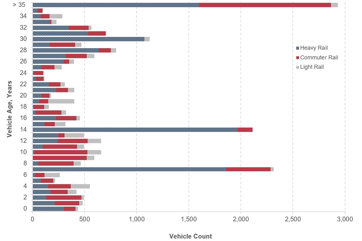
Source: Transit Economic Requirements Model (TERM).

---

Exhibit 6-30: Age Distribution of Hybrid Rail, Streetcar, and Other Rail Transit Vehicles, 2014

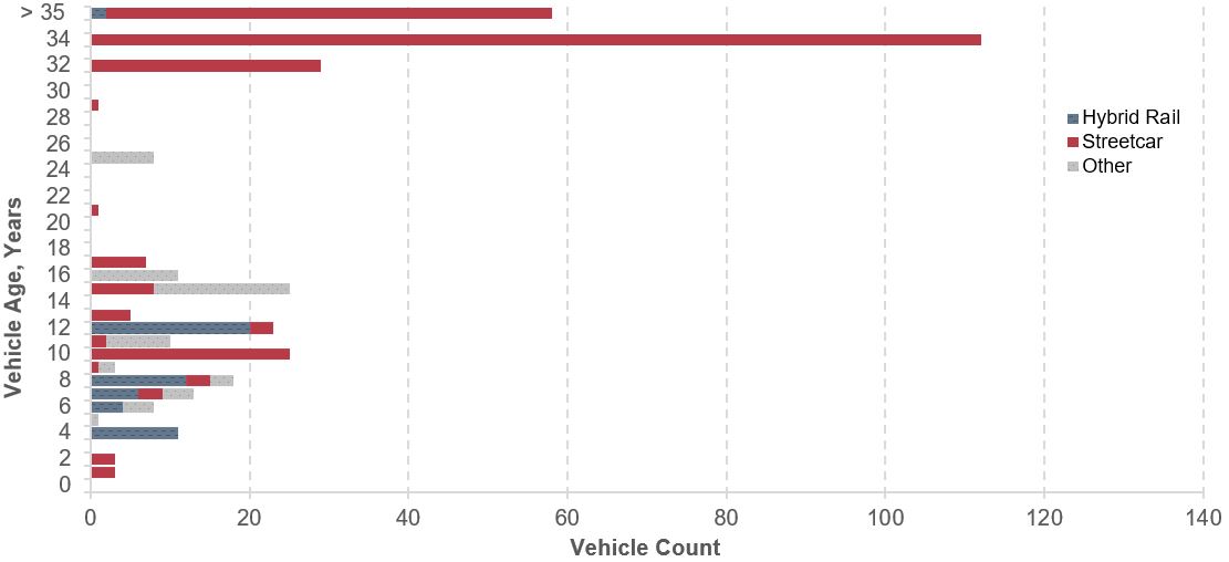
Source: Transit Economic Requirements Model (TERM).

Assets associated with nonvehicle transit rail can be divided into four general categories: guideway elements, systems, stations, and facilities. TERM estimates of the condition distribution for each category are shown in Exhibit 6-31.

---

Exhibit 6-31: Distribution of Asset Physical Conditions by Asset Type for All Rail

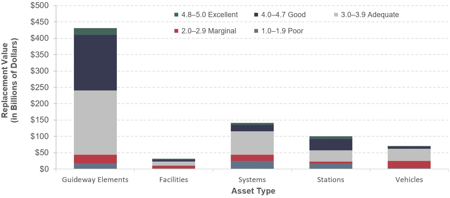
Source: Transit Economic Requirements Model (TERM) and National Transit Database.

The largest category by replacement value is guideway elements. These elements consist of tracks, ties, switches, ballasts, tunnels, and elevated structures. The replacement value of this category is $431.1 billion, of which $17.4 billion is rated below condition 2.0 (4 percent) and $27.0 billion is rated between conditions 2.0 and 3.0.

Although maintaining these assets is among the larger expenses associated with rail transit, FTA does not collect detailed data on these elements, in part because the elements are difficult to categorize into discrete sections having common life expectancies. Service life for track, for example, depends highly on the amount of use it receives and its location.

Systems, which consist of power, communication, and train control equipment, have a replacement value of $141.5 billion, of which $24.7 billion is rated below condition 2.0 (17 percent) and $19.1 billion is rated between conditions 2.0 and 3.0. This category is another for which many assets are difficult to characterize in terms of standard types and life expectancies. As a result, FTA has only limited data from which to make needs projections.

Stations have a replacement value of $100.0 billion, of which $16.3 billion is rated below condition 2.0 and $6.5 billion is rated between conditions 2.0 and 3.0.

Facilities, consisting principally of maintenance and administration buildings, have a replacement value of $31.5 billion. The value of facilities rated below condition 2.0 is $2.4 billion, and that of facilities between conditions 2.0 and 3.0 is $8.3 billion.

Almost half of rail transit vehicles are in heavy rail systems. Heavy rail represents $522.6 billion (67 percent) of the total transit rail replacement cost of $774.9 billion. Heavy rail serves some of the Nation’s oldest and largest transit systems, including Boston, New York, Washington, San Francisco, Philadelphia, and Chicago.

The condition distribution of heavy rail assets, which represent the largest share of U.S. rail transit assets, is shown in Exhibit 6-32. Exhibit 6-33 shows the average age and condition of nonvehicle transit assets for fixed-route bus and rail modes reported for 2014.

While Exhibit 6-31 depicts the replacement value of national transit assets by category for rail modes, Exhibit 6-33 provides additional data such as average fleet age, average condition, and percentage of assets below the SGR threshold (rating below 2.5).

---

Exhibit 6-32: Distribution of Asset Physical Conditions by Asset Type for Heavy Rail

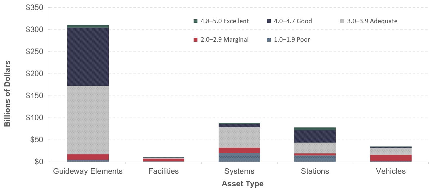
Source: Transit Economic Requirements Model (TERM) and National Transit Database.

---

Exhibit 6-33: Non-Vehicle Transit Assets: Age and Condition, 2014

Category	Mode Type	Average Age	Avg. Condition	Percent Below Condition 2.5
Facilities	Rail	35.9	3.3	24%
	Fixed-Route Bus	30.8	3.2	7%
	All	32.9	3.2	14%
Guideway Elements	Rail	66.4	3.0	37%
	Fixed-Route Bus	25.1	4.4	7%
	All	65.6	3.0	37%
Stations	Rail	59.0	2.8	54%
	Fixed-Route Bus	23.9	3.2	27%
	All	57.4	2.8	53%
Systems	Rail	33.7	3.2	21%
	Fixed-Route Bus	24.6	3.4	19%
	All	33.1	3.2	21%

Source: Transit Economics Requirement Model (TERM).

The preceding discussion in this Section focused on the value of transit assets in excellent, good, adequate, marginal, or poor condition. The remaining discussion considers the value of assets in SGR versus those assets with deferred reinvestment needs (i.e., a reinvestment “backlog”). This discussion is intended to help facilitate an understanding of the similarities and differences between the condition distributions presented above with the proportions of assets in or out of SGR. This assessment of the value of transit assets in SGR versus assets in the reinvestment backlog was estimated using FTA’s TERM. Specifically, this analysis determines the value of assets in the reinvestment backlog as follows:

• Replaceable Assets: The estimated value of replaceable assets that may require replacement (are below condition 2.5) plus the value of replaceable assets with deferred rehabilitation and capital maintenance needs.
• Nonreplaceable Assets: The estimated value of nonreplaceable assets with deferred rehabilitation and capital maintenance needs.

Exhibit 6-34 presents the value of transit assets in SGR versus those assets in the reinvestment backlog, segmented by asset type. Based on this analysis, roughly $790 billion or 89 percent of all transit assets are in SGR, with the remaining $98.0 billion (13 percent) making up the reinvestment backlog. The backlog consists of $21.5 billion for guideway, $11.0 billion for facilities, $30.6 billion for systems, $19.1 billion for stations, and $15.8 billion for vehicles. Comparing Exhibit 6-34 with the condition distribution in Exhibit 6-22 helps to highlight the relationship between these two charts. Specifically, the value of assets in the backlog for each asset category exceeds the value of assets below condition 2.0 in Exhibit 6-22. This is as expected, as the backlog includes the value of all replaceable assets below condition 2.5 plus a (much smaller) amount for assets with deferred rehabilitation and capital maintenance needs.

---

Exhibit 6-34: Value of U.S. Transit Assets in SGR vs Backlog by Asset Type

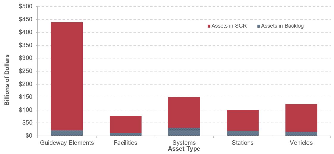
Source: Transit Economic Requirements Model (TERM) and National Transit Database.

Exhibit 6-35 and Exhibit 6-36 provide a similar presentation of transit assets in SGR versus those in the backlog, here segmented by fixed-route bus and all rail assets, respectively. Exhibit 6-35 highlights the fact that 86 percent of fixed-route-bus asset value and 78 percent of the bus backlog are concentrated in vehicle fleet and facilities holdings. The value of rail assets in SGR and the backlog are similar to those found for all transit assets in Exhibit 6-36, demonstrating rail’s large share of total transit asset value. Based on these two charts, the reinvestment backlog constitutes 13 percent of fixed-route-bus asset holdings and 11 percent of rail asset holdings (by value).

---

Exhibit 6-35: Value of U.S. Transit Assets in SGR vs Backlog by Asset Type for Fixed-Route Bus

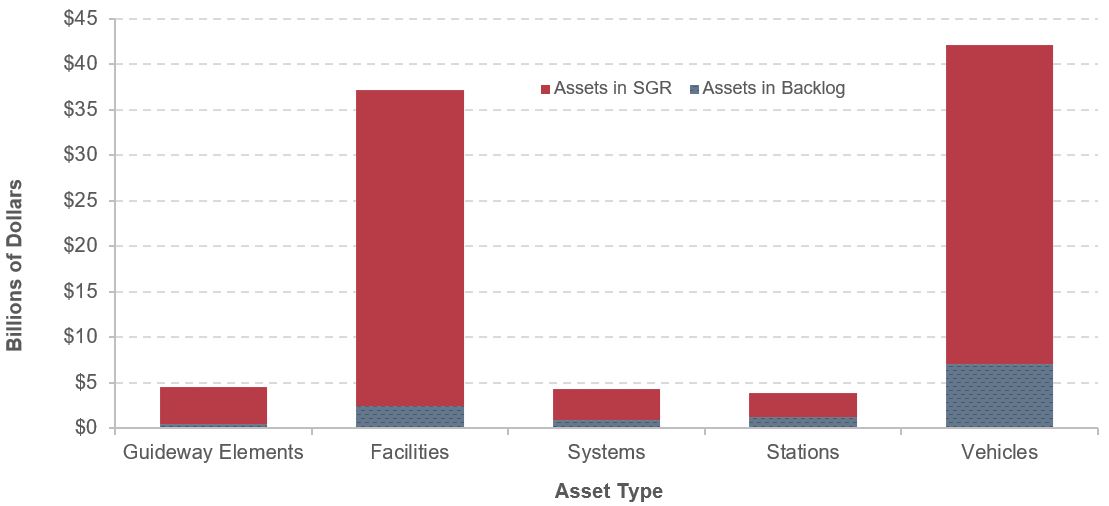
Source: Transit Economic Requirements Model (TERM) and National Transit Database.

---

Exhibit 6-36: Value of U.S. Transit Assets in SGR vs Backlog by Asset Type for Rail

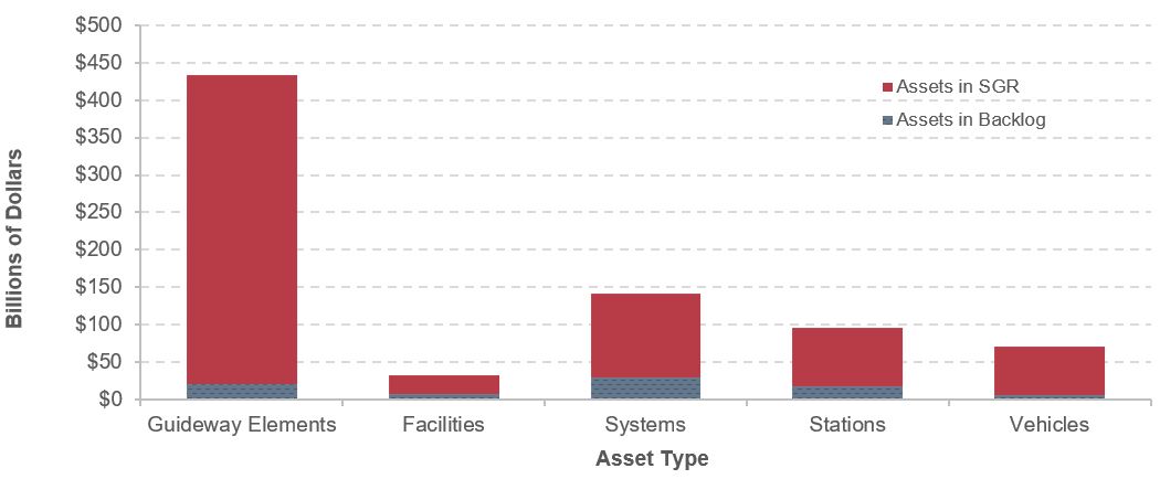
Sources: Transit Economic Requirements Model (TERM); National Transit Database.