

Part II: Investing for the Future
- Introduction
- Capital Investment Scenarios
- Highway and Bridge Investment Scenarios
- Transit Investment Scenarios
- Comparisons Between Report Editions
- The Economic Approach to Transportation Investment Analysis
- Chapter 7: Capital Investment Scenarios
- Chapter 8: Supplemental Analysis
- Chapter 9: Sensitivity Analysis
- Chapter 10: Impacts of Investment
Introduction
Chapters 7 through 10 present and analyze several possible scenarios for future capital investment in highways, bridges, and transit. In each of these 20-year scenarios, the investment level is an estimate of the spending that would be required to achieve a certain specified level of system performance. This report does not attempt to address issues of cost responsibility. The scenarios do not address how much different levels of government might contribute to funding the investment, nor do they directly address the potential contributions of different public or private revenue sources.
The four investment-related chapters in Part II measure investment levels in constant 2014 dollars, except where noted otherwise. The chapters consider scenarios for investment from 2015 through 2034 that are geared toward maintaining some indicator of physical condition or operational performance at its 2014 level, or achieving some objective linked to benefits versus costs. The average annual investment level over the 20 years from 2015 through 2034 is presented for each analyzed scenario.
Chapter 7, Selected Capital Investment Scenarios, defines the core scenarios and examines the associated projections for condition and performance. It also explains how the projections are derived by supplementing the modeling results with assumptions about nonmodeled investment. The analyzed scenarios are intended to be illustrative and do not represent comprehensive alternative transportation policies; the U.S. Department of Transportation (DOT) does not endorse any scenario as a target level of investment.
Chapter 8, Supplemental Scenario Analysis, explores some implications of the scenarios presented in Chapter 7 and contains some additional policy-oriented analyses. As part of this analysis, highway projections from previous editions of the C&P Report are compared with actual outcomes to illuminate the value and limitations of the projections presented in this edition. Chapter 9, Sensitivity Analysis, explores the impacts on scenario projections of changes to several key assumptions, such as the discount rate and the future rate of growth in travel demand.
Lastly, Chapter 10, Impacts of Investment, explores the impacts of alternative levels of possible future investment on various indicators of conditions and performance and explains the derivation of the scenario projections from results obtained with the models that have been developed over the years to support the C&P Report. These models have evolved over time to incorporate recent research, new data sources, and improved estimation techniques; their current versions are described in Appendices A (highways), B (bridges), and C (transit). Even collectively, however, their scope does not cover all capital investment in these types of surface transportation infrastructure.
The combination of engineering and economic analysis in this part of the C&P Report is consistent with the movement of transportation agencies toward asset and performance management, value engineering, and greater consideration of cost-effectiveness in decision-making. The economic approach to transportation investment is discussed at the end of this section.
Capital Investment Scenarios
The projections for the 20-year capital investment scenarios shown in this report reflect complex technical analyses that attempt to predict the potential impacts of capital investment on the future conditions and performance of the transportation system. These scenarios are illustrative, and DOT does not endorse any of them as a target level of investment. Where practical, supplemental information is included to describe the impacts of other possible investment levels.
The investment scenarios project the impact that particular levels of combined Federal, State, local, and private investment might have on the overall conditions and performance of highways, bridges, and transit. Although Chapter 2 provides information on the portions of highway investment that have come from different levels of government in the past, the report makes no specific recommendations about what these portions, or the portion from the private sector, should be in the future.
The system condition and performance projections in this report’s capital investment scenarios represent what could be achievable assuming a particular level of investment, rather than what would be achieved. The models used to develop the projections generally assume that, when funding is constrained, the benefit-cost ratio (BCR) establishes the order of precedence among potential capital projects, with projects having higher BCRs selected first. In actual practice, the BCR generally omits some types of benefits and costs because of difficulties in valuing them monetarily, and these other benefits and costs can and do affect project selection. In addition, actual project selection can be guided by political or other considerations outside benefit-cost analysis.
A last prefatory caveat is that “investment” refers throughout this report to capital spending, which does not include spending on maintenance (although in popular parlance, capital spending on rehabilitation is sometimes described as “maintenance”). Additional discussion of the distinction between capital and maintenance spending is contained in Chapter 2 of this report.
Highway and Bridge Investment Scenarios
Projections for future conditions and performance under alternative potential levels of investment in highways and bridges combined are presented as scenarios in Chapter 7 and developed from projections in Chapter 10 using separate models and techniques for highway preservation and capacity expansion and for bridge preservation. Investments in bridge repair, rehabilitation, and replacement are modeled by the National Bridge Investment Analysis System (NBIAS); those in capacity expansion and the highway resurfacing and reconstruction component of system rehabilitation are modeled by the Highway Economic Requirements System (HERS). Some elements of highway investment spending are modeled by neither HERS nor NBIAS. Chapter 7 factors these elements into the investment levels associated with each scenario using scaling procedures external to the models. The scenario investment levels are estimates of the amount of future capital spending required to meet the performance goals specified in the scenarios.
For all Federal-aid highways, the National Highway System, and the Interstate System separately, Chapter 10 presents model-based projections of highway conditions and performance under alternative assumptions about future investment levels. Chapter 7 also maintains this disaggregation in the projections for the Improve Conditions and Performance scenario described below. However, due to data limitations, the scenario projections in Chapter 7 also rely heavily on assumptions to incorporate nonmodeled investment. Although the NBIAS database includes information on all bridges, the Highway Performance Monitoring System (HPMS) database, on which the HERS model relies, includes detailed information only on Federal-aid highways; for the scenarios based on all roads, non-model-based estimates must be generated for roads functionally classified as rural minor collectors, rural local, or urban local. In addition, HERS lacks information that would be needed to model some types of investment, such as safety-focused projects (e.g., adding rumble strips).
The Sustain 2014 Spending scenario projects the potential impacts of sustaining capital spending at 2014 base-year levels in constant-dollar terms over the 20-year period 2015 through 2034. The Maintain Conditions and Performance scenario also assumes that capital spending in constant-dollar terms remains flat between 2015 and 2034—not at the 2014 level, but at the level that would result in selected performance indicators having the same values in 2034 as in 2014. For this edition of the C&P Report, the HERS component of the scenario is defined as the lowest level of investment required at a minimum to maintain each of two performance indicators—average pavement roughness and average delay per vehicle mile traveled (VMT)—at their base-year level or better. For the NBIAS component, the benchmark performance indicator is the percentage of deck area on bridges that is in poor condition.
What are the implications of the Improve Conditions and Performance scenario for non-capital spending?
Exhibit 2-6 (see Chapter 2) shows that maintenance and other non-capital costs of highways are substantial, comprising roughly half of all highway expenditures. Since capital investments in infrastructure generally have implications for future maintenance requirements, one important question about the Improve Conditions and Performance scenario is how this capital investment level would affect future maintenance costs.
In the HERS model, maintenance spending per mile is estimated based on pavement condition and strength, with maintenance costs rising as pavement condition declines. Maintenance costs are also estimated to increase in proportion to the number of lanes. As such, increases in capital spending on rehabilitation projects generally reduce the need for future maintenance spending, by improving pavement condition. Conversely, capacity expansion projects increase the number of lanes that need to be maintained and thus imply higher future maintenance costs, all other things being equal. The NBIAS model similarly estimates higher maintenance costs as bridge condition declines, and NBIAS does not simulate capacity expansion projects.
The Improve Conditions and Performance scenario includes roughly three times more annual spending on system rehabilitation improvements (see Chapter 7, Exhibit 7-4). Because of this weighting toward rehabilitation, the overall impact of the scenario is to reduce rather than increase future maintenance costs. Specifically, HERS estimates that the Improve Conditions and Performance scenario would reduce maintenance costs from an initial level of $1,393 per mile to $1,052 per mile at the end of the 20-year forecast period, a reduction of 24.5 percent.
Other non-capital costs, such as administration and highway patrol, are not captured in the HERS model, but do not necessarily vary strongly with changes in capital investment. The increased investment under the Improve Conditions and Performance scenario would likely result in additional planning costs, though once a project reaches the preliminary engineering stage such costs would be included as part of the estimated capital investment. To the extent that increased spending under this scenario were financed through the issuance of bonds, this would tend to increase future bond interest and bond redemption expenses.
The investment levels for the Improve Conditions and Performance scenario are estimates of what would be needed to fund all cost-beneficial highway and bridge improvements. This scenario represents an “investment ceiling” above which further investment would not be cost-beneficial, even if available funding were unlimited. The portion of this funding that is directed toward pavement and bridge rehabilitation (as opposed to capacity expansion) is described as the State of Good Repair benchmark.
Types of Capital Spending Projected by HERS and NBIAS
The types of investments HERS and NBIAS evaluate can be related to the system of highway functional classification introduced in Chapter 1 and to the broad categories of capital improvements introduced in Chapter 2 (system rehabilitation, system expansion, and system enhancement). NBIAS relies on the National Bridge Inventory (NBI) database, which covers bridges on all highway functional classes and evaluates improvements that generally fall within the system rehabilitation category.
How closely do the types of capital improvements modeled in HERS and NBIAS correspond to the specific capital improvement type categories presented in Chapter 2?
Exhibit 2-12 (see Chapter 2) provides a crosswalk between a series of specific capital improvement types for which data are routinely collected from the States and three major summary categories: system rehabilitation, system expansion, and system enhancement. The types of improvements covered by HERS and NBIAS are assumed to correspond with the system rehabilitation and system expansion categories. As in Exhibit 2-12, HERS splits spending on “reconstruction with added capacity” among these categories.
For some of the detailed categories in Exhibit 2-12, the assumed correspondence is close overall but not exact. In particular, the extent to which HERS covers construction of new roads and bridges is ambiguous. Although not directly modeled in HERS, such investments are often motivated by a desire to alleviate congestion on existing facilities in a corridor, and thus would be captured indirectly by the HERS analysis in the form of additional normal-cost or high-cost lanes. The costs per mile assumed in HERS for high-cost lanes are based on typical costs of tunneling, double-decking, or building parallel routes, depending on the functional class and area population size for the section being analyzed. To the extent that investments in the “new construction” and “new bridge” improvement types identified in Chapter 2 are motivated by desires to encourage economic development or accomplish other goals aside from the reduction of congestion on the existing highway network, such investments would not be captured in the HERS analysis.
Some other comparability issues include:
- Some of the relocation expenditures identified in Exhibit 2-12 may be motivated by considerations beyond those reflected in the curve and grade rating data that HERS uses in computing the benefits of horizontal and vertical realignments.
- The bridge expenditures that Exhibit 2-12 counts as system rehabilitation could include work on bridge approaches and ancillary improvements that NBIAS does not model.
- HERS and NBIAS are assumed not to capture improvements that count as system enhancement spending, including the spending on the “safety” category in Exhibit 2-12. Some safety deficiencies, however, might be addressed as part of broader pavement and capacity improvements modeled in HERS.
- The HERS operations preprocessor described in Appendix A includes capital investments in operations equipment and technology that would fall under the definition of the “traffic management/engineering” improvement type in Chapter 2. These investments are counted among the nonmodeled system enhancements because they are not evaluated within the benefit-cost framework that HERS applies to system preservation and expansion investments.
HERS evaluates pavement improvements—resurfacing or reconstruction—and highway widening; the types of improvements included in these categories roughly correspond to system rehabilitation and system expansion as described in Chapter 2. In estimating the per-mile costs of widening improvements, HERS recognizes a typical number of bridges and other structures that would need modification. Thus, the estimates from HERS are considered to represent system expansion costs for both highways and bridges. Coverage of the HERS analysis is limited, however, to Federal-aid highways, as the Highway Performance Monitoring System (HPMS) sample does not include data for rural minor collectors, rural local roads, or urban local roads.
The term “nonmodeled spending” refers in this report to spending on highway and bridge capital improvements that are not evaluated in HERS or NBIAS; such spending is not included in the analyses presented in Chapter 10, but the capital investment scenarios presented in Chapter 7 are adjusted to account for them. Nonmodeled spending includes capital improvements on highway classes omitted from the HPMS sample and, hence, the HERS model. The development of the future investment scenarios for the highway system as a whole thus required supplementary estimation outside the HERS modeling process.
Nonmodeled spending also includes types of capital expenditures classified in Chapter 2 as system enhancements, which neither HERS nor NBIAS currently evaluates. Although HERS incorporates assumptions about future operations investments, the capital components of which would be classified as system enhancements, the model does not directly evaluate the need for these deployments. In addition, HERS does not identify specific safety-oriented investment opportunities, but instead considers the ancillary safety impacts of capital investments that are directed primarily toward system rehabilitation or capacity expansion. The HPMS database contains no information on the locations of crashes and safety devices, such as guardrails or rumble strips, limiting the model.
Exhibit II-1 shows that, systemwide in 2014, highway capital spending was $105.4 billion. Of that spending, $60.2 billion was for the types of improvement that HERS models, and $14.4 billion was for the types of improvement NBIAS models. The other $30.9 billion, which was for nonmodeled highway capital spending, was divided between system enhancement expenditures and capital improvements to classes of highways not reported in HPMS.
Because the HPMS sample data are available only for Federal-aid highways, the percentage of capital improvements classified as nonmodeled spending is lower for Federal-aid highways than is the case systemwide. Of the $79.3 billion spent by all levels of government on capital improvements to Federal-aid highways in 2014, 75.9 percent was within the scope of HERS, 13.3 percent was within the scope of NBIAS, and 10.8 percent was for spending captured by neither. The percentage distribution differs somewhat for the Interstate System, with a slightly higher share within the scope of HERS and NBIAS (80.3 percent and 12.5 percent, respectively) and a smaller share captured by neither (7.2 percent).
Exhibit II-1: Distribution of 2014 Capital Expenditures by Investment Type
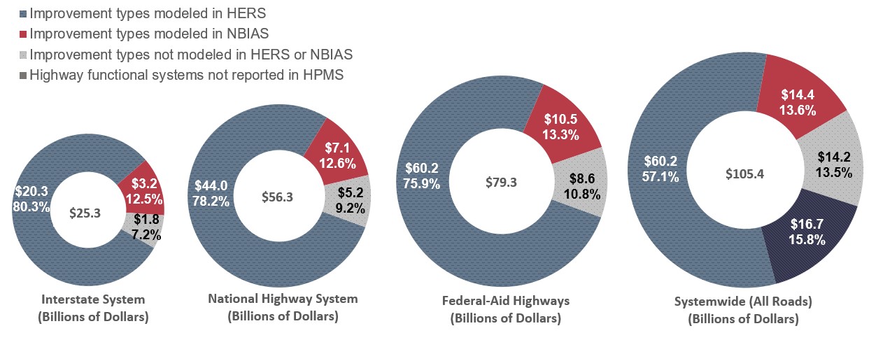
Source: Highway Statistics 2014 (Table SF-12A) and unpublished FHWA data.
Highway Economic Requirements System
Simulations conducted with HERS provide the basis for this report’s analysis of investment in highway resurfacing and reconstruction and for highway and bridge capacity expansion. HERS uses incremental benefit-cost analysis to evaluate highway improvements based on data from HPMS. HPMS includes State-supplied information on current roadway characteristics, conditions, performance, and anticipated future travel growth for a nationwide sample of roughly 120,000 highway sections. HERS analyzes individual sample sections only as a step toward providing results at the national level; the model does not provide definitive improvement recommendations for individual sections.
The frame for which sections are sampled is the TOPS (Table of Potential Samples), in which each section is relatively homogeneous over its length as to traffic volume, geometrics, cross-section, and condition. For each State, the sampling is designed to enable statistically reliable estimation for each urbanized area, and at the statewide level for rural and for small urban areas. For each of these geographic categories, stratified random samples are drawn by traffic volume group. (The sampling methodology is further detailed in the HPMS Field Manual (https://www.fhwa.dot.gov/policyinformation/hpms/fieldmanual/).)
HERS simulations begin with evaluations of the current state of the highway system using data from the HPMS sample. These data provide information on pavements, roadway geometry, traffic volume and composition (percentage of trucks), and other characteristics of the sampled highway sections. For sections with one or more identified deficiencies, the model then considers potential improvements, including resurfacing, reconstruction, alignment improvements, and widening or adding travel lanes. HERS selects the improvement (or combination of improvements) with the greatest net benefits, with benefits defined as reductions in direct highway user costs, agency costs for highway maintenance, and societal costs from vehicle emissions of pollutants. The model allocates investment funding only to those sections for which at least one potential improvement is projected to produce benefits exceeding construction costs.
HERS normally considers highway conditions and performance over a period of 20 years from the base (“current”) year—the most recent year for which HPMS data are available. This analysis period is divided into four equal funding periods. After analyzing the first funding period, HERS updates the database to reflect the projected outcomes of the first period, including the effects of the selected highway improvements. The updated database is then used to analyze conditions and performance in the second period, the database is updated again, and so on through the fourth and final period.
Operations Strategies
HERS considers the impacts of certain types of highway operational improvements that feature intelligent transportation systems. The operations strategies HERS currently evaluates are:
- Freeway management: ramp metering, electronic roadway monitoring, variable message signs, integrated corridor management, variable speed limits, queue warning systems, lane controls.
- Incident management: detection, verification, response.
- Arterial management: upgraded signal control, electronic monitoring, variable message signs.
- Traveler information: 511 systems, advanced in-vehicle navigation systems with real-time traveler information.
In contrast with improvements that expand or rehabilitate highways, HERS does not analyze the benefits and costs of these operational improvements. Thus, the model does not estimate the needs for investment in operational improvements. Instead, a separate preprocessor estimates the impacts of these operations strategies on the performance of highway sections where they are deployed. The analyses presented in this chapter assume a package of investments that continue existing deployment trends. HERS does not currently model applications of various developing vehicle-to-vehicle and vehicle-to-infrastructure communications because it is not yet possible to predict reliably the impacts and patterns of their deployment.
Operations improvements vs. capacity improvements in HERS
Because HERS does not perform benefit-cost analysis for highway operational improvements, the scenarios in the C&P Report simply assume certain strategies for their future deployment. In this edition, the assumption is that deployment will continue at a rate consistent with existing patterns. The previous two editions made the same assumption, but also presented sensitivity analyses that alternatively assumed: (1) a more aggressive deployment strategy over 20 years, and (2) a full deployment strategy (implementing the aggressive deployments over 5 years. The analyses estimated the impacts of these alternatives on the overall levels of scenario spending, including spending on capacity expansion and pavement preservation—which HERS subjects to benefit-cost analysis— and on deployments of operational improvements. In both the Maintain and Improve scenarios, these impacts showed small increases in overall spending in the 2013 C&P Report, and small decreases in the 2015 C&P Report. The differences in estimated spending impacts between the 2013 C&P and 2015 C&P Reports could have many causes, and they are not indications of whether more aggressive deployment of operational improvements would be cost-beneficial.
Travel Demand Elasticity
A key feature of the HERS economic analysis is the influence of the cost of travel on demand for travel. HERS represents this relationship as a travel demand elasticity that relates demand, measured by vehicle miles traveled (VMT), to changes in the average user cost of travel that result from either: (1) changes in highway conditions and performance as measured by travel delay, pavement condition, and crash costs, relative to base year levels; the elasticity mechanism reduces travel demand when these changes are for the worse (e.g., an increase in travel delay) and increase travel demand when they are improvements (e.g., better pavement condition); or (2) deviations from the price projections built into the baseline demand forecasts. This report considers the latter deviations only in Chapter 9 where one of the sensitivity tests alters the projections for motor fuel prices.
HERS also allows the induced demand predicted through the elasticity mechanism to influence the cost of travel to highway users. For example, a 10-percent reduction in travel cost per mile would be predicted to induce a 6 percent increase in VMT in the short term, and a larger increase—just under 12 percent—5 years later, as travelers are able to make additional responses to the change in costs. On congested sections of highway, the initial congestion relief afforded by an increase in capacity will reduce the average user cost per VMT, which in turn will stimulate demand for travel; this increased demand will in turn reverse some of the initial congestion relief. The elasticity feature operates likewise with respect to improvements in pavement quality by allowing for induced traffic that adds to pavement wear. (Conversely, an initial increase in user costs can start a causal chain with effects in the opposite direction.) By capturing these offsets to initial impacts on highway user costs, HERS can estimate the net impacts.
National Bridge Investment Analysis System
The scenario estimates relating to bridge repair and replacement shown in this report are derived primarily from NBIAS. NBIAS can synthesize element-level data from the general condition ratings reported for individual bridges in the NBI. The analyses presented in this report are based on synthesized element-level data. Examples of bridge elements include the bridge deck, a steel girder used for supporting the deck, a concrete pier cap on which girders are placed, a concrete column used for supporting the pier cap, or a bridge railing.
NBIAS uses a probabilistic approach to model bridge deterioration for each synthesized bridge element. It relies on a set of transition probabilities to project the likelihood that an element will deteriorate from one condition state to another over a given period. This information, along with details on the cost of maintenance, repair, and rehabilitation (MR&R) actions, is used to predict lifecycle costs of maintaining existing bridges, and to develop MR&R policies specifying what MR&R action to perform based on the existing condition of a bridge element. Notwithstanding the use of the term “maintenance”, the MR&R actions are actually capital improvements, and preventive maintenance (e.g., cleaning scuppers, washing bridges) is not modeled.
Another key input to the model is the overall objective assumed for MR&R policies. The State of Good Repair strategy, although the most aggressive of the available MR&R policies, generates results more consistent with agency practices and recent trends in bridge conditions compared with the other three strategies evaluated (see Appendix B). Therefore, the State of Good Repair strategy has been adopted for use in the baseline analyses presented in this chapter and in Chapter 7.
The State of Good Repair strategy aims to improve all bridges to good condition that can be sustained through ongoing investment. MR&R investment is front-loaded under the State of Good Repair strategy, as large MR&R investments are required in the early years of the forecast period to improve bridge conditions, while smaller MR&R investments are needed in the later years to sustain bridge conditions. Under this analysis, replacement of a bridge is recommended if a bridge evaluation results in lower lifecycle costs compared with the recommended MR&R work.
To estimate functional improvement needs, NBIAS applies a set of improvement standards and costs to each bridge in the NBI. The system then identifies potential improvements—such as widening existing bridge lanes, raising bridges to increase vertical clearances, and strengthening bridges to increase load-carrying capacity—and evaluates their potential benefits and costs. NBIAS evaluates potential bridge replacements by comparing their benefits and costs with what could be achieved through MR&R work alone. Appendix B discusses NBIAS in detail.
Transit Investment Scenarios
The transit section of Chapter 10 evaluates the impact of varying levels of capital investment on various measures of condition and performance, while the transit section of Chapter 7 provides a more in-depth analysis of specific investment scenarios.
The Sustain 2014 Spending scenario projects the potential impacts of sustaining preservation and expansion spending at 2014 base-year levels in constant-dollar terms over the 20-year period of 2015 through 2034. The scenario applies benefit-cost analysis to prioritize investments within this constrained budget target.
The State of Good Repair benchmark projects the level of investment needed to bring all assets to a state of good repair over the next 20 years, defined as asset condition ratings of 2.5 or higher on a 5-point scale (Chapter 6 discusses these ratings). This scenario does not apply a benefit-cost test and focuses solely on the preservation of existing assets.
The Low-Growth and High-Growth scenarios each add a system expansion component to the system preservation needs associated with the State of Good Repair benchmark. The goal of these scenarios is to preserve existing assets and expand the transit asset base to support projected ridership growth over 20 years, based on forecasts linked to the average annual growth experienced between 1999 and 2014. The Low-Growth scenario projects ridership growth at 0.3 percent per year below the historical trend (over 15 years), while the High-Growth scenario incorporates a more extensive expansion of the existing transit asset base to support ridership growth at 0.3 percent per year above the historical trend. Both scenarios incorporate a benefit-cost test for evaluating potential investments; thus, their system preservation components are somewhat smaller than the level identified in the State of Good Repair benchmark.
Types of Capital Spending Projected by TERM
TERM is an analysis tool that uses algorithms based on engineering and economic concepts to forecast total capital investment needs for the U.S. transit industry through a 20-year time horizon. Specifically, TERM is designed to forecast the following types of investment needs:
- Preservation: The level of investment in the rehabilitation and replacement of existing transit capital assets required to attain specific investment goals (e.g., to attain a state of good repair [SGR]) subject to potentially limited capital funding.
- Expansion: The level of investment in the expansion of transit fleets, facilities, and rail networks required to support projected growth in transit demand (i.e., to maintain performance at current levels as demand for service increases).
Recent Investment in Transit Preservation and Expansion
As reported to NTD, the level of transit capital expenditures peaked in 2009 at $16.8 billion, experienced a slight decrease in 2011 to $15.6 billion, and increased again in 2014 to $17.7 billion (see Exhibit II-2). Although the annual transit capital expenditures averaged $15.2 billion from 2004 to 2014, expenditures averaged $16.8 billion in the most recent 5 years of NTD reporting (2010–2014). Furthermore, even though capital expenditures for preservation purposes in 2014 increased by $0.5 billion relative to prior-year levels, capital expenditures for expansion purposes remained the same as in 2013.
Exhibit II-2: Annual Transit Capital Expenditures, 2004–2014
| Year | (Billions of Current-Year Dollars) | (Billions of Constant 2014 Dollars) | ||||
|---|---|---|---|---|---|---|
| Preservation | Expansion | Total | Preservation | Expansion | Total | |
| 2004 | $9.4 | $3.2 | $12.6 | $11.8 | $4.0 | $15.8 |
| 2005 | $9.0 | $2.9 | $11.8 | $10.9 | $3.5 | $14.3 |
| 2006 | $9.2 | $3.5 | $12.7 | $10.8 | $4.1 | $14.9 |
| 2007 | $9.6 | $4.0 | $13.6 | $10.9 | $4.6 | $15.5 |
| 2008 | $11.0 | $5.1 | $16.0 | $12.1 | $5.6 | $17.6 |
| 2009 | $11.3 | $5.5 | $16.8 | $12.5 | $6.1 | $18.6 |
| 2010 | $10.3 | $6.2 | $16.6 | $11.2 | $6.8 | $18.0 |
| 2011 | $9.9 | $5.7 | $15.6 | $10.5 | $6.0 | $16.5 |
| 2012 | $9.7 | $7.1 | $16.8 | $10.0 | $7.4 | $17.4 |
| 2013 | $10.8 | $6.4 | $17.1 | $10.9 | $6.5 | $17.4 |
| 2014 | $11.0 | $6.4 | $17.4 | $11.0 | $6.4 | $17.4 |
| Average | $10.1 | $5.1 | $15.2 | $11.1 | $5.5 | $16.7 |
Source: National Transit Database.
Preservation Investments
TERM estimates current and future preservation investment needs by first assessing the age and current condition of the Nation’s existing stock of transit assets. (The results of this analysis were presented in Chapter 6 of this report.) TERM then uses this information to assess both current reinvestment needs (i.e., the reinvestment backlog) and the expected level of ongoing investment required to meet the life-cycle needs of the Nation’s transit assets over the next 20 years, including all required rehabilitation and replacement activities.
Condition-Based Reinvestment
Rather than relying on age alone in assessing the timing and cost of current and future reinvestment activities, TERM uses a set of empirical asset deterioration curves that estimate asset condition (both current and future) as a function of asset type, age, past rehabilitation activities, and, depending on asset type, past maintenance and utilization levels. An asset’s estimated condition at the start of each year over the 20-year forecast horizon determines the timing of specific rehabilitation and replacement activities. Asset condition declines as the asset ages, triggering reinvestment events at different levels of deterioration and ultimately leading to outright replacement.
Financial Constraints, the Investment Backlog, and Future Conditions
TERM is designed to estimate investment needs with or without annual capital funding constraints. When run without funding constraints, TERM estimates the total level of investment required to complete all rehabilitation and replacement needs the model identifies at the time those investment needs come due (hence, with unconstrained analyses after any initial deferred investment is addressed, investment backlog is not appreciable). In contrast, when TERM is run in a financially constrained mode, sufficient funding might not be available to cover the reinvestment needs of all assets. In this case, some reinvestment activities would be deferred until sufficient funds become available. The lack of funds to address all reinvestment needs for some or all of the 20 years of the model forecast results in varying levels of investment backlog during this period. Most analyses presented in this chapter were completed using funding constraints. Similarly, TERM’s ability to estimate asset conditions—both current and future—allows for assessment of how future asset conditions are likely to improve or decline given varying levels of capital reinvestment. Finally, note that TERM’s benefit-cost analysis is used to determine the order in which reinvestment activities are completed when funding capacity is limited, with investments having the highest benefit-cost ratios addressed first.
Expansion Investments
In addition to ongoing reinvestment in existing assets, most transit agencies invest in the expansion of their vehicle fleets, maintenance facilities, fixed guideway, and other assets. Investments in expansion assets can be considered as serving two distinct purposes. First, the demand for transit services typically increases over time in line with population growth, employment, and other factors. To maintain current levels of performance in the face of expanding demand, transit operators must similarly expand the capacity of their services (e.g., by increasing the number of vehicles in their fleets). Failure to accommodate this demand would result in increased vehicle crowding, increased dwell times at passenger stops, and decreased operating speeds for existing services. Second, transit operators also invest in expansion projects with the aim of improving current service performance. Such improvements include capital expansion projects (e.g., a new light rail segment) to reduce vehicle crowding or increase average operating speeds. TERM is designed to assess investment needs and impacts for both types of expansion investments.
To assess the level of investment required to maintain existing service quality, TERM estimates the rate of growth in transit vehicle fleets required to maintain current vehicle occupancy levels given the projected growth rate in transit passenger miles. In addition to assessing the level of investment in new fleet vehicles required to support this growth, TERM forecasts investments in the expansion of other assets needed to support projected fleet growth, including bus maintenance facilities and—in the case of rail systems—additional investment in guideway, track work, stations, maintenance facilities, train control, and traction power systems. Asset expansion investment needs are assessed on a mode-by-mode basis for all agencies reporting to NTD. Cost-benefit constraints, however, prevent TERM from investing in asset expansion for those agency modes having lower ridership (per vehicle) than the national average.
Comparisons Between Report Editions
The base year of the analysis typically advances two years between successive editions of this biennial report. During this period, changes in many real-world factors can affect the investment scenario estimates. Among these factors are construction costs and other prices, conditions and performance of the highway and transit systems, expansion of the system asset base, and changes in technology (such as improvements in motor vehicle fuel economy). Although relevant to all scenarios, the implications of these changes are particularly significant for scenarios aimed at maintaining base-year conditions. Comparability across C&P Report editions is also limited by changes over time in analytical tools, data sets used in generating the scenarios, and scenario definitions. For example, the projected rates of highway traffic growth—key inputs to HERS and NBIAS—have changed considerably. These and other key changes are discussed in Chapters 7, 8, and 10.
The Economic Approach to Transportation Investment Analysis
The economic approach to transportation investment entails analysis and comparison of benefits and costs. Investments that yield benefits for which the values exceed their costs increase societal welfare and are thus considered “economically efficient,” or “cost-beneficial.” While the 1968 National Highway Needs Report to Congress began as a mere “wish list” of State highway needs, the approach to estimating investment needs in the C&P Report has become more economic and in other ways more sophisticated over the subsequent editions.
As the focus of national highway investment changed from system expansion to management of the existing system during the 1970s, national engineering standards were defined and applied to identify system deficiencies, and the investments necessary to remedy these deficiencies were estimated. By the end of the decade, a comprehensive database, the HPMS, had been developed to enable monitoring of highway system conditions and performance nationwide.
In the early 1980s, a sophisticated simulation model, the HPMS Analytical Process (HPMS-AP), became available to evaluate the impact of alternative investment strategies on system conditions and performance. The procedures used in HPMS-AP were based on engineering principles. Engineering standards were applied to determine which system attributes were considered deficient, and improvement option packages were developed using standard engineering countermeasures for given deficiencies, but without consideration of comparative economic benefits and costs.
In 1988, the Federal Highway Administration embarked on a long-term research and development effort to produce an alternative simulation procedure combining engineering principles with economic analysis. The product of this effort, the HERS model, was first used to develop one of the two highway investment scenarios presented in the 1995 C&P Report. In subsequent reports, HERS has been used to develop all the highway investment scenarios.
Executive Order 12893, “Principles for Federal Infrastructure Investments,” issued on January 26, 1994, directs that Federal infrastructure investments should be based on a systematic analysis of expected benefits and costs. This order provided additional momentum for the shift toward developing analytical tools that incorporate economic analysis into the evaluation of investment requirements.
In the 1997 C&P Report, the Federal Transit Administration introduced the Transit Economics Requirements Model (TERM). TERM incorporates benefit-cost analysis into its determination of transit investment levels. The 2002 C&P Report incorporated economic analysis into bridge investment modeling for the first time with the introduction of NBIAS.
The Economic Approach in Theory and Practice
Effective use of the economic approach to investment appraisal requires adequate consideration of the range of possible benefits and costs and of the range of possible investment alternatives.
Which Benefits and Costs Should Be Considered?
A comprehensive benefit-cost analysis of a transportation investment considers all impacts of potential significance for society and values them in monetary terms, to the extent feasible. For some types of impacts, monetary valuation is facilitated by the existence of observable market prices. Such prices are generally available for inputs to the provision of transportation infrastructure, such as concrete for building highways or buses purchased for a transit system. The same is true for some types of benefits from transportation investments, such as savings in business travel time, which are conventionally valued at a measure of average hourly labor cost of the travelers.
For some other types of impacts for which market prices are not directly observable, monetary values can be reasonably inferred from behavior or expressed preferences. In this category are savings in nonbusiness travel time and reductions in risk of crash-related fatality or other injury. As discussed in Chapter 9 (under “Value of a Statistical Life”), what is inferred is the amount that people typically would be willing to pay per unit of improvement, such as, per hour of nonbusiness travel time saved. These values are combined with estimates of the magnitude of the improvement (or, as may happen, deterioration).
For other impacts, monetary valuation may not be possible because of problems with reliably estimating the magnitude of the improvement, placing a monetary value on the improvement, or both. Even when possible, reliable monetary valuation may require time and effort that would be out of proportion to the likely importance of the impact concerned. Benefit-cost analyses of transportation investments thus typically will omit valuing certain impacts that are difficult to monetize but, nevertheless, could be of interest.
Each of the models used in this report—HERS, NBIAS, and TERM—omits various types of investment impacts from its benefit-cost analyses. To some extent, this omission reflects the national coverage of the models’ primary databases. Although consistent with this report’s focus on the Nation’s highways and transit systems, such broad geographic coverage requires some sacrifice of detail to stay within feasible budgets for data collection. In the future, technological progress in data collection and growing demand for data for performance management systems for transportation infrastructure likely will yield national databases that are more comprehensive and of better quality.
In addition, DOT will continue to explore other avenues for addressing impacts not captured by the suite of models used for the C&P Report. One approach is to have the models represent impacts in ways that are sufficiently simplified to demand no more data than are available. This approach was taken to represent within HERS the impacts of traffic disruptions resulting from road construction. Another effect the DOT models do not consider, but which could be significant for some transportation investments, is the boost to economic competition that results when travel times within and between regions are lessened. Faced with stiffer competition from rivals in other locations, producers may become more efficient and reduce their prices.
What Alternatives Should Be Analyzed?
Benefit-cost analyses of transportation investments need to include a sufficiently broad range of investment alternatives to be able to identify which is optimal. For transit and highway projects, this evaluation can entail consideration of cross-modal alternatives. Transit and highway projects can be complementary, as when the addition of high-occupancy toll lanes to a freeway allows for new or improved express bus services; they can also be substitutes, as when construction of a light rail line lessens the demand for travel on a parallel freeway. In contrast, both HERS and TERM focus on investment in just one mode. To incorporate a cross-modal perspective properly would require a major investment of time and resources, entailing major changes to the benefit-cost methodologies and the addition of considerable detail to the supporting databases. (As was noted earlier, the models’ databases necessarily sacrifice detail to make national-level coverage feasible.) Opportunities for future development of HERS, TERM, and NBIAS, including efforts to allow feedback between the models, were discussed in Appendix D of the 2013 C&P Report.
Beyond related cross-modal investment possibilities, economic evaluations of investments in highways or transit should also attempt to consider related public choices, such as policies for travel demand management and local zoning, or investment in other infrastructure. Several previous editions of the C&P Report presented HERS modeling of highway investment combined with systemwide highway congestion pricing. Although the results indicated that pricing could substantially reduce the amount of highway investment that would be cost-beneficial, a review of the methodology in 2010 revealed significant limitations, which reflected in part the lack of transportation network detail in the HPMS database.
A more limited form of congestion pricing is tolling on designated express lanes within a full access-controlled highway. When the tolling includes a discount or exemption for high-occupancy vehicles, such facilities are termed HOT (High-Occupancy Toll) lanes. Over the past three decades, tolled express lanes have been implemented in urban areas across the United States. Future versions of the HERS model could include a capability to analyze the costs and benefits of tolled express lanes and their effects on investment needs.
Measurement of Costs and Benefits in “Constant Dollars”
Benefit-cost analyses normally measure all benefits and costs in “constant dollars,” that is, at the prices prevailing in some base year, typically near the year when the analysis is released. Future price changes can be difficult to forecast, and benefits and costs measured in base-year prices ensure consistency when comparing benefits and costs.
In the simplest form of constant-dollar measurement, any quantity is converted to a dollar value at that quantity’s base-year price. Future savings in gallons of gasoline, for example, are monetized at the average price per gallon of gasoline in the base year (with the price measured net of excise tax, as in HERS). This approach, still quite common in benefit-cost analysis, was the general practice in pre-2008 editions of the C&P Report. It assumes any future inflation will change all prices in equal proportion, so that the ratios among prices will remain constant at their base-year levels.
An alternative approach to constant dollar measurement factors in future changes in relative prices. This is warranted when such changes are significant, pertain to the relative price of a quantity important to the analysis, and can be predicted with sufficient confidence. What constitutes sufficient confidence is a judgment call, but some predictions carry official weight. The Energy Information Administration’s Annual Energy Outlook forecasts changes in constant dollar motor-fuel prices up to 25 years out. Starting with the 2008 C&P Report, the highway investment scenarios have incorporated these forecasts.
Uncertainty in Transportation Investment Modeling
The three investment analysis models used in this report are deterministic, not probabilistic, in that they provide a single projected value of total investment for a given scenario rather than a range of likely values. As a result, only general statements can be made about the element of uncertainty in these projections, based on the characteristics of the process used to develop them; specific information about confidence intervals cannot be developed. As was indicated previously, the analysis in Chapter 9 of this edition of the C&P Report enables uncertainty to be addressed by analyzing the sensitivity of the scenario projections to variation in the underlying parameters (e.g., discount rates, value of time saved, statistical value of lives saved). As much as possible, the range of variation considered in these tests corresponds to the range considered plausible in the corresponding research literature or to ranges recommended in authoritative guidance. The sensitivity tests address only some of the elements of uncertainty in the scenario projections. In some cases, the uncertainty extends beyond the value of a model parameter to the entire specification of the equations in which the parameters are embedded.
The relative level of uncertainty differs among the various projections made in this report. The projections for absolute levels of condition and performance indicators entail more uncertainty than do the relative differences among these levels according to an assumed level of investment. For example, if speed limits were changed in the future, contrary to the HERS modeling assumption of no change from the base-year speed limits, this could reduce the accuracy of the model’s projections for average speed. At the same time, projections of how the amount of future investments in highways affects average speed could be relatively accurate. Although investments in highway capacity expansion increase average speed, the increase will occur primarily under conditions of congestion when average speeds can be well below even the current speed limit. Under such conditions, an increase in the speed limit might have a negligible effect on the congestion reduction benefits of adding lanes.